Determination of the optimal nano-hexapod’s stiffness

1. Spindle Rotation Speed
2. Micro-Station Compliance Effect
3. Payload “Impedance” Effect
4. Total Change of dynamics

As shown before, many parameters other than the nano-hexapod itself do influence the plant dynamics:

The micro-station compliance (studied here)
The payload mass and dynamical properties (studied here and here)
The experimental conditions, mainly the spindle rotation speed (studied here)

As seen before, the stiffness of the nano-hexapod greatly influence the effect of such parameters.

We wish here to see if we can determine an optimal stiffness of the nano-hexapod such that:

Section 1: the change of its dynamics due to the spindle rotation speed is acceptable
Section 2: the support compliance dynamics is not much present in the nano-hexapod dynamics
Section 3: the change of payload impedance has acceptable effect on the plant dynamics

The overall goal is to design a nano-hexapod that will allow the highest possible control bandwidth.

1 Spindle Rotation Speed

In this section, we look at the effect of the spindle rotation speed on the plant dynamics.

The rotation speed will have an effect due to the Coriolis effect.

1.1 Initialization

We initialize all the stages with the default parameters.

initializeGround();
initializeGranite();
initializeTy();
initializeRy();
initializeRz();
initializeMicroHexapod();
initializeAxisc();
initializeMirror();

We use a sample mass of 10kg.

initializeSample('mass', 10);

We don’t include disturbances in this model as it adds complexity to the simulations and does not alter the obtained dynamics. We however include gravity.

initializeSimscapeConfiguration('gravity', true);
initializeDisturbances('enable', false);
initializeLoggingConfiguration('log', 'none');
initializeController();

1.2 Identification when rotating at maximum speed

We identify the dynamics for the following spindle rotation speeds Rz_rpm:

Rz_rpm = linspace(0, 60, 6);

And for the following nano-hexapod actuator stiffness Ks:

Ks = logspace(3,9,7); % [N/m]

1.3 Change of dynamics

We plot the change of dynamics due to the change of the spindle rotation speed (from 0rpm to 60rpm):

Figure 2: from actuator force \(\tau\) to force sensor \(\tau_m\) (IFF plant)
Figure 3: from actuator force \(\tau\) to actuator relative displacement \(d\mathcal{L}\) (Decentralized positioning plant)
Figure 4: from force in the task space \(\mathcal{F}_x\) to sample displacement \(\mathcal{X}_x\) (Centralized positioning plant)
Figure 5: from force in the task space \(\mathcal{F}_x\) to sample displacement \(\mathcal{X}_y\) (coupling of the centralized positioning plant)

Figure 1: Root Locus plot for IFF control when not rotating (in red) and when rotating at 60rpm (in blue) for 4 different nano-hexapod stiffnesses (png, pdf)

Figure 2: Change of dynamics from actuator \(\tau\) to actuator force sensor \(\tau_m\) for a spindle rotation speed from 0rpm to 60rpm (png, pdf)

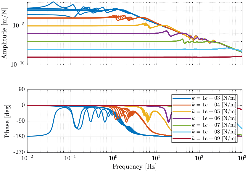
Figure 3: Change of dynamics from actuator force \(\tau\) to actuator displacement \(d\mathcal{L}\) for a spindle rotation speed from 0rpm to 60rpm (png, pdf)

Figure 4: Change of dynamics from force \(\mathcal{F}_x\) to displacement \(\mathcal{X}_x\) for a spindle rotation speed from 0rpm to 60rpm (png, pdf)

Figure 5: Change of Coupling from force \(\mathcal{F}_x\) to displacement \(\mathcal{X}_y\) for a spindle rotation speed from 0rpm to 60rpm (png, pdf)

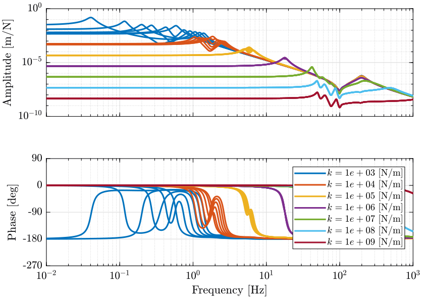
The leg stiffness should be at higher than \(k_i = 10^4\ [N/m]\) such that the main resonance frequency does not shift too much when rotating. For the coupling, it is more difficult to conclude about the minimum required leg stiffness.

Note that we can use very soft nano-hexapod if we limit the spindle rotating speed.

2 Micro-Station Compliance Effect

take the 6dof compliance of the micro-station
simple model + uncertainty

2.1 Identification of the micro-station compliance

We initialize all the stages with the default parameters.

initializeGround();
initializeGranite();
initializeTy();
initializeRy();
initializeRz();
initializeMicroHexapod('type', 'compliance');

We put nothing on top of the micro-hexapod.

initializeAxisc('type', 'none');
initializeMirror('type', 'none');
initializeNanoHexapod('type', 'none');
initializeSample('type', 'none');

And we identify the dynamics from forces/torques applied on the micro-hexapod top platform to the motion of the micro-hexapod top platform at the same point. The diagonal element of the identified Micro-Station compliance matrix are shown in Figure 6.

Figure 6: Identified Compliance of the Micro-Station (png, pdf)

2.2 Identification of the dynamics with a rigid micro-station

We now identify the dynamics when the micro-station is rigid. This is equivalent of identifying the dynamics of the nano-hexapod when fixed to a rigid ground. We also choose the sample to be rigid and to have a mass of 10kg.

initializeSample('type', 'rigid', 'mass', 10);

As before, we identify the dynamics for the following actuator stiffnesses:

Ks = logspace(3,9,7); % [N/m]

2.3 Identification of the dynamics with a flexible micro-station

We now initialize all the micro-station stages to be flexible. And we identify the dynamics of the nano-hexapod.

2.4 Obtained Dynamics

We plot the change of dynamics due to the compliance of the Micro-Station. The solid curves are corresponding to the nano-hexapod without the micro-station, and the dashed curves with the micro-station:

Figure 7: from actuator force \(\tau\) to force sensor \(\tau_m\) (IFF plant)
Figure 8: from actuator force \(\tau\) to actuator relative displacement \(d\mathcal{L}\) (Decentralized positioning plant)
Figure 9: from force in the task space \(\mathcal{F}_x\) to sample displacement \(\mathcal{X}_x\) (Centralized positioning plant)
Figure 10: from force in the task space \(\mathcal{F}_z\) to sample displacement \(\mathcal{X}_z\) (Centralized positioning plant)

Figure 7: Change of dynamics from actuator \(\tau\) to actuator force sensor \(\tau_m\) due to the micro-station compliance (png, pdf)

Figure 8: Change of dynamics from actuator force \(\tau\) to actuator displacement \(d\mathcal{L}\) due to the micro-station compliance (png, pdf)

Figure 9: Change of dynamics from force \(\mathcal{F}_x\) to displacement \(\mathcal{X}_x\) due to the micro-station compliance (png, pdf)

Figure 10: Change of dynamics from force \(\mathcal{F}_z\) to displacement \(\mathcal{X}_z\) due to the micro-station compliance (png, pdf)

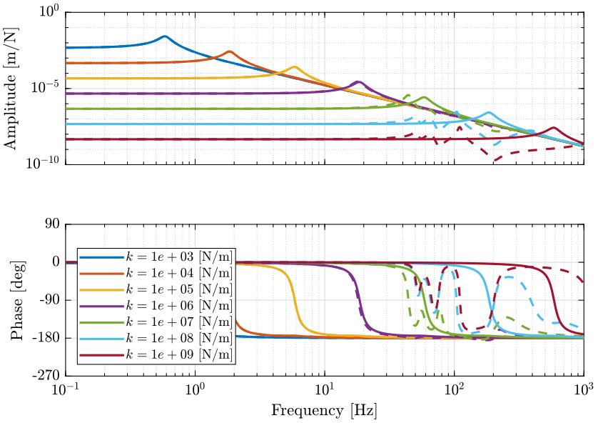
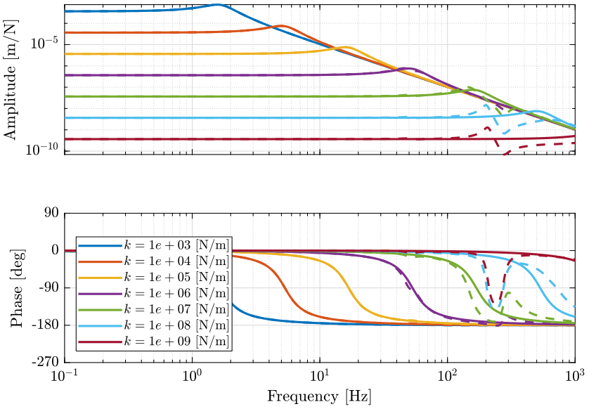
The dynamics of the nano-hexapod is not affected by the micro-station dynamics (compliance) when the stiffness of the legs is less than \(10^6\ [N/m]\). When the nano-hexapod is stiff (\(k>10^7\ [N/m]\)), the compliance of the micro-station appears in the primary plant.

3 Payload “Impedance” Effect

3.1 Initialization

We initialize all the stages with the default parameters. We don’t include disturbances in this model as it adds complexity to the simulations and does not alter the obtained dynamics. :exports none

initializeDisturbances('enable', false);

We set the controller type to Open-Loop, and we do not need to log any signal.

initializeSimscapeConfiguration('gravity', true);
initializeController();
initializeLoggingConfiguration('log', 'none');
initializeReferences();

3.2 Identification of the dynamics while change the payload dynamics

We make the following change of payload dynamics:

Change of mass: from 1kg to 50kg
Change of resonance frequency: from 50Hz to 500Hz
The damping ratio of the payload is fixed to \(\xi = 0.2\)

We identify the dynamics for the following payload masses Ms and nano-hexapod leg’s stiffnesses Ks:

Ms = [1, 20, 50]; % [Kg]
Ks = logspace(3,9,7); % [N/m]

We then identify the dynamics for the following payload resonance frequencies Fs:

Fs = [50, 200, 500]; % [Hz]

3.3 Change of dynamics for the primary controller

3.3.1 Frequency variation

We here compare the dynamics for the same payload mass, but different stiffness resulting in different resonance frequency of the payload:

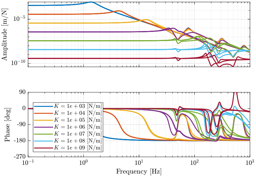
Figure 11: dynamics from a force \(\mathcal{F}_z\) applied in the task space in the vertical direction to the vertical displacement of the sample \(\mathcal{X}_z\) for both a very soft and a very stiff nano-hexapod.
Figure 12: same, but for all tested nano-hexapod stiffnesses

We can see two mass lines for the soft nano-hexapod (Figure 11):

The first mass line corresponds to \(\frac{1}{(m_n + m_p)s^2}\) where \(m_p = 10\ [kg]\) is the mass of the payload and \(m_n = 15\ [Kg]\) is the mass of the nano-hexapod top platform and attached mirror
The second mass line corresponds to \(\frac{1}{m_n s^2}\)
The zero corresponds to the resonance of the payload alone (fixed nano-hexapod’s top platform)

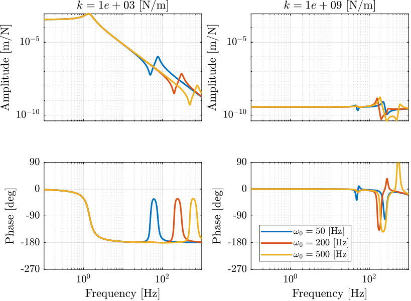
Figure 11: Dynamics from \(\mathcal{F}_z\) to \(\mathcal{X}_z\) for varying payload resonance frequency, both for a soft nano-hexapod and a stiff nano-hexapod

Figure 12: Dynamics from \(\mathcal{F}_z\) to \(\mathcal{X}_z\) for varying payload resonance frequency (png, pdf)

3.3.2 Mass variation

We here compare the dynamics for different payload mass with the same resonance frequency (100Hz):

Figure 13: dynamics from a force \(\mathcal{F}_z\) applied in the task space in the vertical direction to the vertical displacement of the sample \(\mathcal{X}_z\) for both a very soft and a very stiff nano-hexapod.
Figure 14: same, but for all tested nano-hexapod stiffnesses

We can see here that for the soft nano-hexapod:

the first resonance \(\omega_n\) is changing with the mass of the payload as \(\omega_n = \sqrt{\frac{k_n}{m_p + m_n}}\) with \(k_p\) the stiffness of the nano-hexapod, \(m_p\) the payload’s mass and \(m_n\) the mass of the nano-hexapod top platform
the first mass line corresponding to \(\frac{1}{(m_p + m_n)s^2}\) is changing with the payload mass
the zero at 100Hz is not changing as it corresponds to the resonance of the payload itself
the second mass line does not change

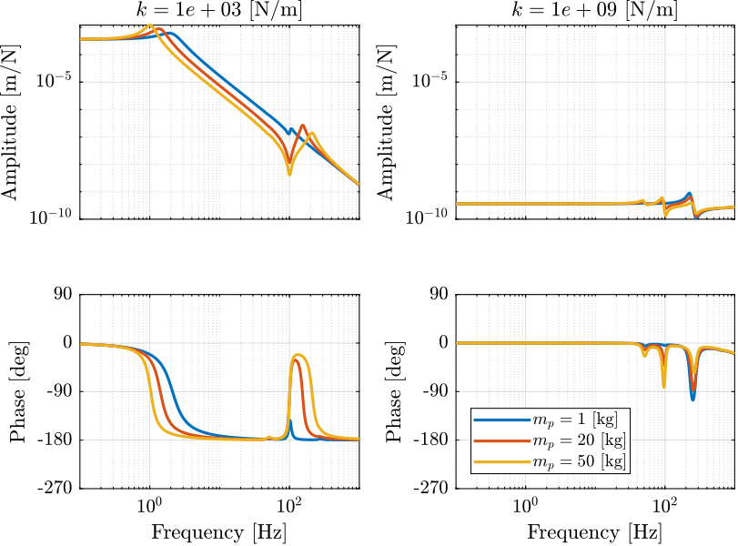
Figure 13: Dynamics from \(\mathcal{F}_z\) to \(\mathcal{X}_z\) for varying payload mass, both for a soft nano-hexapod and a stiff nano-hexapod

Figure 14: Dynamics from \(\mathcal{F}_z\) to \(\mathcal{X}_z\) for varying payload mass (png, pdf)

3.3.3 Total variation

We now plot the total change of dynamics due to change of the payload (Figures 15 and 16):

mass from 1kg to 50kg
main resonance from 50Hz to 500Hz

Figure 15: Dynamics from \(\mathcal{F}_z\) to \(\mathcal{X}_z\) for varying payload dynamics, both for a soft nano-hexapod and a stiff nano-hexapod (png, pdf)

Figure 16: Dynamics from \(\mathcal{F}_z\) to \(\mathcal{X}_z\) for varying payload dynamics, both for a soft nano-hexapod and a stiff nano-hexapod (png, pdf)

4 Total Change of dynamics

We now consider the total change of nano-hexapod dynamics due to:

Gk_wz_err - Change of spindle rotation speed
Gf_err and Gm_err - Change of payload resonance
Gmf_err and Gmr_err - Micro-Station compliance

The obtained dynamics are shown:

Figure 17 for a stiffness \(k = 10^3\ [N/m]\)
Figure 18 for a stiffness \(k = 10^5\ [N/m]\)
Figure 19 for a stiffness \(k = 10^7\ [N/m]\)
Figure 20 for a stiffness \(k = 10^9\ [N/m]\)

And finally, in Figures 21 and 22 are shown an animation of the change of dynamics with the nano-hexapod’s stiffness.

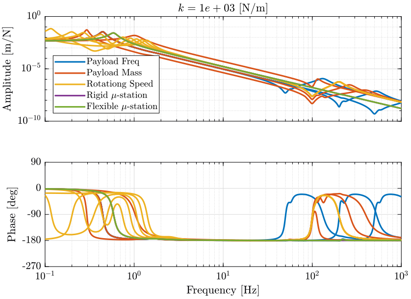
Figure 17: Total variation of the dynamics from \(\mathcal{F}_x\) to \(\mathcal{X}_x\). Nano-hexapod leg’s stiffness is equal to \(k = 10^3\ [N/m]\) (png, pdf)

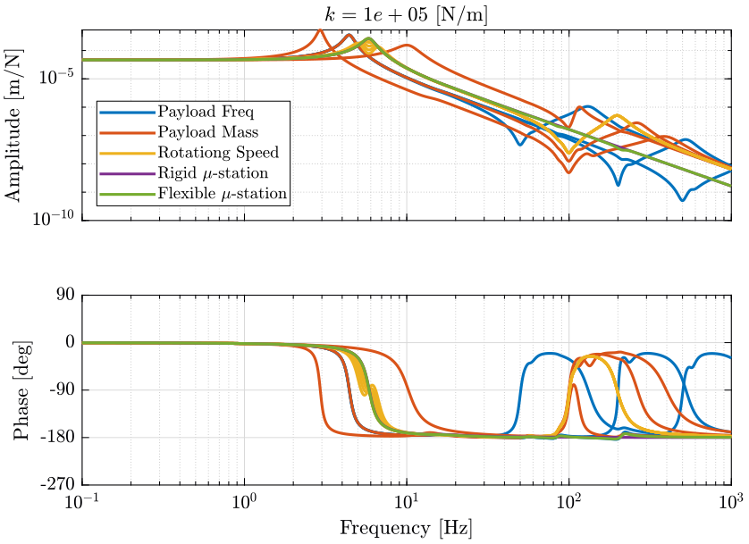
Figure 18: Total variation of the dynamics from \(\mathcal{F}_x\) to \(\mathcal{X}_x\). Nano-hexapod leg’s stiffness is equal to \(k = 10^5\ [N/m]\) (png, pdf)

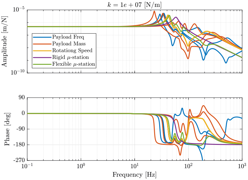
Figure 19: Total variation of the dynamics from \(\mathcal{F}_x\) to \(\mathcal{X}_x\). Nano-hexapod leg’s stiffness is equal to \(k = 10^7\ [N/m]\) (png, pdf)

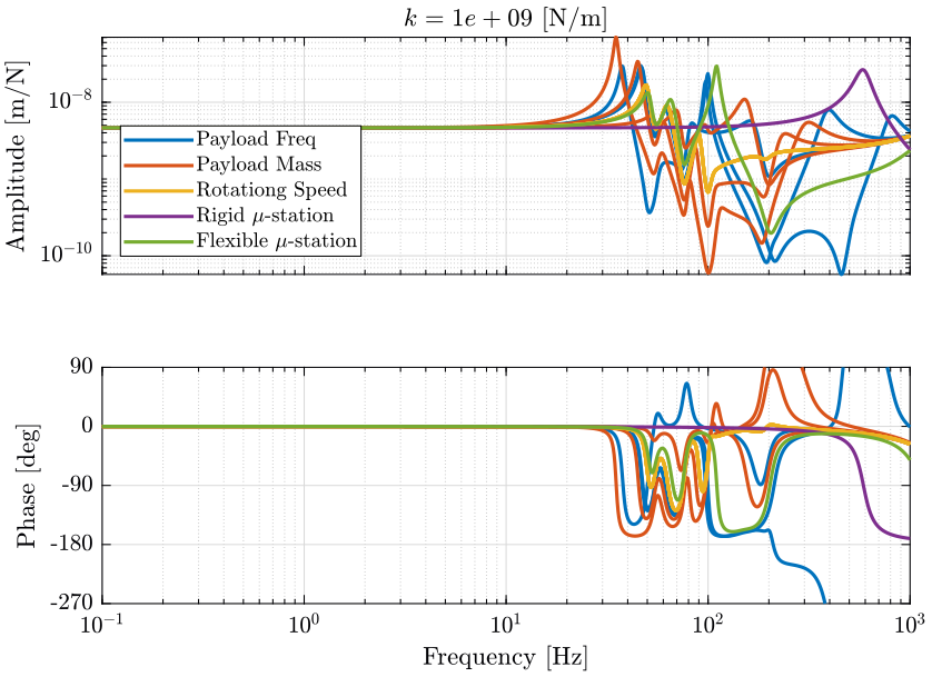
Figure 20: Total variation of the dynamics from \(\mathcal{F}_x\) to \(\mathcal{X}_x\). Nano-hexapod leg’s stiffness is equal to \(k = 10^9\ [N/m]\) (png, pdf)

Figure 21: Variability of the dynamics from \(\mathcal{F}_x\) to \(\mathcal{X}_x\) with varying nano-hexapod stiffness

Figure 22: Variability of the dynamics from \(\mathcal{F}_x\) to \(\mathcal{X}_x\) with varying nano-hexapod stiffness