Identification of the disturbances
Table of Contents
The goal here is to extract the Power Spectral Density of the sources of perturbation.
The sources of perturbations are (schematically shown in figure 1):
- \(D_w\): Ground Motion
- Parasitic forces applied in the system when scanning with the Translation Stage and the Spindle (\(F_{rz}\) and \(F_{ty}\)). These forces can be due to imperfect guiding for instance.
Because we cannot measure directly the perturbation forces, we have the measure the effect of those perturbations on the system (in terms of velocity for instance using geophones, \(D\) on figure 1) and then, using a model, compute the forces that induced such velocity.
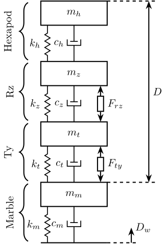
Figure 1: Schematic of the Micro Station and the sources of disturbance
This file is divided in the following sections:
- Section 1: the simscape model used here is presented
- Section 2: transfer functions from the disturbance forces to the relative velocity of the hexapod with respect to the granite are computed using the Simscape Model representing the experimental setup
- Section 3: the bode plot of those transfer functions are shown
- Section 4: the measured PSD of the effect of the disturbances are shown
- Section 5: from the model and the measured PSD, the PSD of the disturbance forces are computed
- Section 6: with the computed PSD, the noise budget of the system is done
1 Simscape Model
The following Simscape model of the micro-station is the same model used for the dynamical analysis. However, we here constrain all the stage to only move in the vertical direction.
We add disturbances forces in the vertical direction for the Translation Stage and the Spindle. Also, we measure the absolute displacement of the granite and of the top platform of the Hexapod.
We load the configuration and we set a small StopTime.
load('mat/conf_simulink.mat');
set_param(conf_simulink, 'StopTime', '0.5');
We initialize all the stages without the sample nor the nano-hexapod. The obtained system corresponds to the status micro-station when the vibration measurements were conducted.
initializeGround();
initializeGranite('type', 'modal-analysis');
initializeTy();
initializeRy();
initializeRz();
initializeMicroHexapod('type', 'modal-analysis');
initializeAxisc('type', 'none');
initializeMirror('type', 'none');
initializeNanoHexapod('type', 'none');
initializeSample('type', 'none');
Open Loop Control.
initializeController('type', 'open-loop');
We don’t need gravity here.
initializeSimscapeConfiguration('gravity', false);
We log the signals.
initializeLoggingConfiguration('log', 'all');
2 Identification
The transfer functions from the disturbance forces to the relative velocity of the hexapod with respect to the granite are computed using the Simscape Model representing the experimental setup with the code below.
%% Name of the Simulink File
mdl = 'nass_model';

%% Micro-Hexapod
clear io; io_i = 1;
io(io_i) = linio([mdl, '/Disturbances'], 1, 'openinput', [], 'Dwz'); io_i = io_i + 1; % Vertical Ground Motion
io(io_i) = linio([mdl, '/Disturbances'], 1, 'openinput', [], 'Fty_z'); io_i = io_i + 1; % Parasitic force Ty
io(io_i) = linio([mdl, '/Disturbances'], 1, 'openinput', [], 'Frz_z'); io_i = io_i + 1; % Parasitic force Rz

io(io_i) = linio([mdl, '/Micro-Station/Granite/Modal Analysis/accelerometer'], 1, 'openoutput'); io_i = io_i + 1; % Absolute motion - Granite
io(io_i) = linio([mdl, '/Micro-Station/Micro Hexapod/Modal Analysis/accelerometer'],  1, 'openoutput'); io_i = io_i + 1; % Absolute Motion - Hexapod

% Run the linearization
G = linearize(mdl, io, 0);
We Take only the outputs corresponding to the vertical acceleration.
G = G([3,9], :);

% Input/Output names
G.InputName  = {'Dw', 'Fty', 'Frz'};
G.OutputName = {'Agm', 'Ahm'};
We integrate 1 time the output to have the velocity and we substract the absolute velocities to have the relative velocity.
G = (1/s)*tf([-1, 1])*G;

% Input/Output names
G.InputName  = {'Dw', 'Fty', 'Frz'};
G.OutputName = {'Vm'};
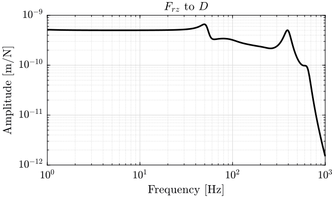
3 Sensitivity to Disturbances
The obtained sensitivity to disturbances are shown bellow:


4 Power Spectral Density of the effect of the disturbances
The Power Spectral Densities of the relative velocity between the hexapod and the marble in \([(m/s)^2/Hz]\) are loaded for the following sources of disturbance:
- Slip Ring Rotation (\(F_{r_z}\))
- Scan of the translation stage (effect in the vertical direction and in the horizontal direction)
Also, the Ground Motion is measured.
gm  = load('./mat/psd_gm.mat', 'f', 'psd_gm');
rz  = load('./mat/pxsp_r.mat', 'f', 'pxsp_r');
tyz = load('./mat/pxz_ty_r.mat', 'f', 'pxz_ty_r');
tyx = load('./mat/pxe_ty_r.mat', 'f', 'pxe_ty_r');
Because some 50Hz and harmonics were present in the ground motion measurement, we remove these peaks with the following code:
f0s = [50, 100, 150, 200, 250, 350, 450];
for f0 = f0s
    i = find(gm.f > f0-0.5 & gm.f < f0+0.5);
    gm.psd_gm(i) = linspace(gm.psd_gm(i(1)), gm.psd_gm(i(end)), length(i));
end
We now compute the relative velocity between the hexapod and the granite due to ground motion.
gm.psd_rv = gm.psd_gm.*abs(squeeze(freqresp(G('Vm', 'Dw'), gm.f, 'Hz'))).^2;
The Power Spectral Density of the relative motion and velocity of the hexapod with respect to the granite are shown in figures 5 and 6.
The Cumulative Amplitude Spectrum of the relative motion is shown in figure 7.
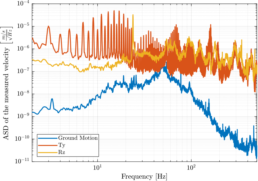
Figure 5: Amplitude Spectral Density of the relative velocity of the hexapod with respect to the granite due to different sources of perturbation (png, pdf)

Figure 6: Amplitude Spectral Density of the relative displacement of the hexapod with respect to the granite due to different sources of perturbation (png, pdf)

Figure 7: Cumulative Amplitude Spectrum of the relative motion due to different sources of perturbation (png, pdf)
From Figure 7, we can see that the translation stage and the rotation stage have almost the same effect on the position error. Also, the ground motion has a relatively negligible effect on the position error.
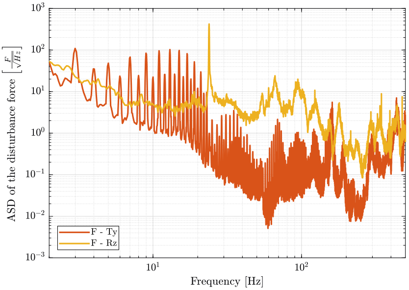
5 Compute the Power Spectral Density of the disturbance force
Using the extracted transfer functions from the disturbance force to the relative motion of the hexapod with respect to the granite (section 3) and using the measured PSD of the relative motion (section 4), we can compute the PSD of the disturbance force.
This is done below.
rz.psd_f  = rz.pxsp_r./abs(squeeze(freqresp(G('Vm', 'Frz'), rz.f, 'Hz'))).^2;
tyz.psd_f = tyz.pxz_ty_r./abs(squeeze(freqresp(G('Vm', 'Fty'), tyz.f, 'Hz'))).^2;
The obtained amplitude spectral densities of the disturbance forces are shown in Figure 8.
6 Noise Budget
From the obtained spectral density of the disturbance sources, we can compute the resulting relative motion of the Hexapod with respect to the granite using the model.
This is equivalent as doing the inverse that was done in the previous section. This is done in order to verify that this is coherent with the measurements.
The power spectral density of the relative motion is computed below and the result is shown in Figure 9. We can see that this is exactly the same as the Figure 6.
psd_gm_d = gm.psd_gm.*abs(squeeze(freqresp(G('Vm', 'Dw')/s, gm.f, 'Hz'))).^2;
psd_ty_d = tyz.psd_f.*abs(squeeze(freqresp(G('Vm', 'Fty')/s, tyz.f, 'Hz'))).^2;
psd_rz_d = rz.psd_f.*abs(squeeze(freqresp(G('Vm', 'Frz')/s, rz.f, 'Hz'))).^2;

7 Save
The PSD of the disturbance force are now saved for further analysis.
dist_f = struct();

dist_f.f = gm.f; % Frequency Vector [Hz]

dist_f.psd_gm = gm.psd_gm; % Power Spectral Density of the Ground Motion [m^2/Hz]
dist_f.psd_ty = tyz.psd_f; % Power Spectral Density of the force induced by the Ty stage in the Z direction [N^2/Hz]
dist_f.psd_rz = rz.psd_f; % Power Spectral Density of the force induced by the Rz stage in the Z direction [N^2/Hz]

save('./mat/dist_psd.mat', 'dist_f');
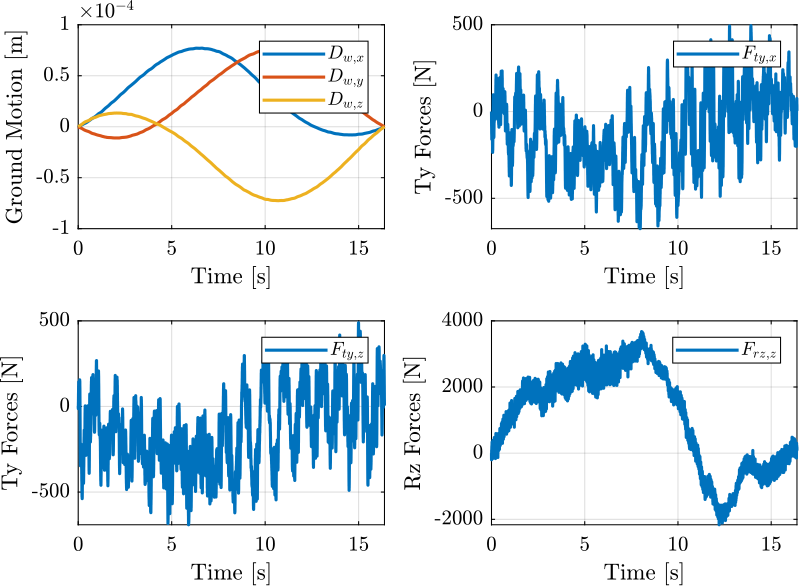
8 Time Domain Disturbances
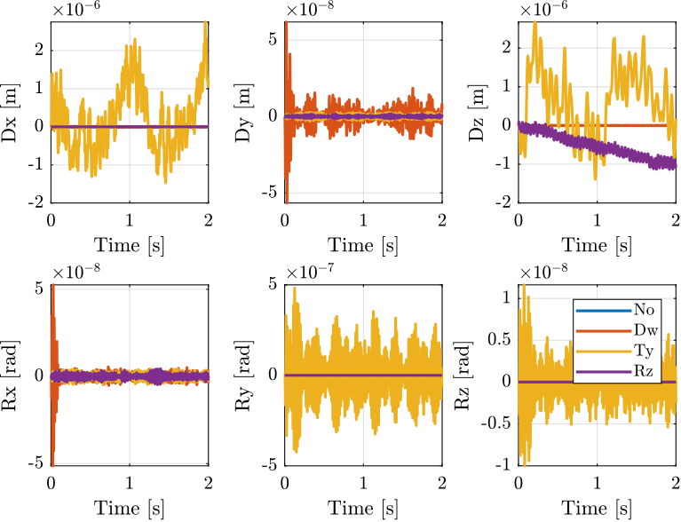
9 Time Domain Effect of Disturbances
9.1 Initialization of the Experiment
We initialize all the stages with the default parameters.
initializeGround();
initializeGranite();
initializeTy();
initializeRy();
initializeRz();
initializeMicroHexapod();
initializeAxisc();
initializeMirror();
The nano-hexapod is a piezoelectric hexapod and the sample has a mass of 50kg.
initializeNanoHexapod('type', 'rigid');
initializeSample('mass', 1);
initializeReferences();
initializeController('type', 'open-loop');
initializeSimscapeConfiguration('gravity', false);
initializeLoggingConfiguration('log', 'all');
load('mat/conf_simulink.mat');
set_param(conf_simulink, 'StopTime', '2');
9.2 Simulations
No disturbances:
initializeDisturbances('enable', false);
sim('nass_model');
sim_no = simout;
Ground Motion:
initializeDisturbances('Fty_x', false, 'Fty_z', false, 'Frz_z', false);
sim('nass_model');
sim_gm = simout;
Translation Stage Vibrations:
initializeDisturbances('Dwx', false, 'Dwy', false, 'Dwz', false, 'Frz_z', false);
sim('nass_model');
sim_ty = simout;
Rotation Stage Vibrations:
initializeDisturbances('Dwx', false, 'Dwy', false, 'Dwz', false, 'Fty_x', false, 'Fty_z', false);
sim('nass_model');
sim_rz = simout;