Decentralize control to add virtual mass
Table of Contents
1 Initialization
initializeGround();
initializeGranite();
initializeTy();
initializeRy();
initializeRz();
initializeMicroHexapod();
initializeAxisc();
initializeMirror();

initializeSimscapeConfiguration();
initializeDisturbances('enable', false);
initializeLoggingConfiguration('log', 'none');

initializeController('type', 'hac-dvf');
The nano-hexapod has the following leg’s stiffness and damping.
initializeNanoHexapod('k', 1e5, 'c', 2e2);
We set the stiffness of the payload fixation:
Kp = 1e8; % [N/m]
2 Identification
We identify the system for the following payload masses:
Ms = [1, 10, 50];
Identification of the transfer function from \(\tau\) to \(d\mathcal{L}\). Identification of the Primary plant without virtual add of mass
3 Adding Virtual Mass in the Leg’s Space
3.1 Plant
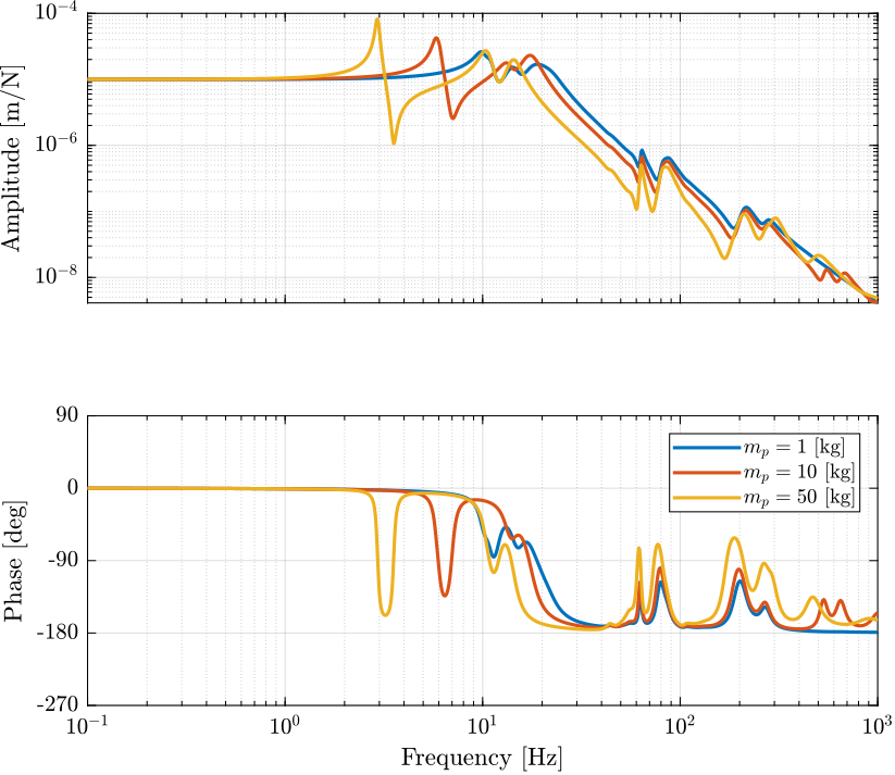
Figure 1: Transfer function from \(\tau_i\) to \(d\mathcal{L}_i\) for three payload masses
3.2 Controller Design
Kdvf = 10*s^2/(1+s/2/pi/500)^2*eye(6);
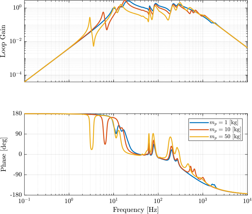
Figure 2: Loop Gain for the addition of virtual mass in the leg’s space
3.3 Identification of the Primary Plant
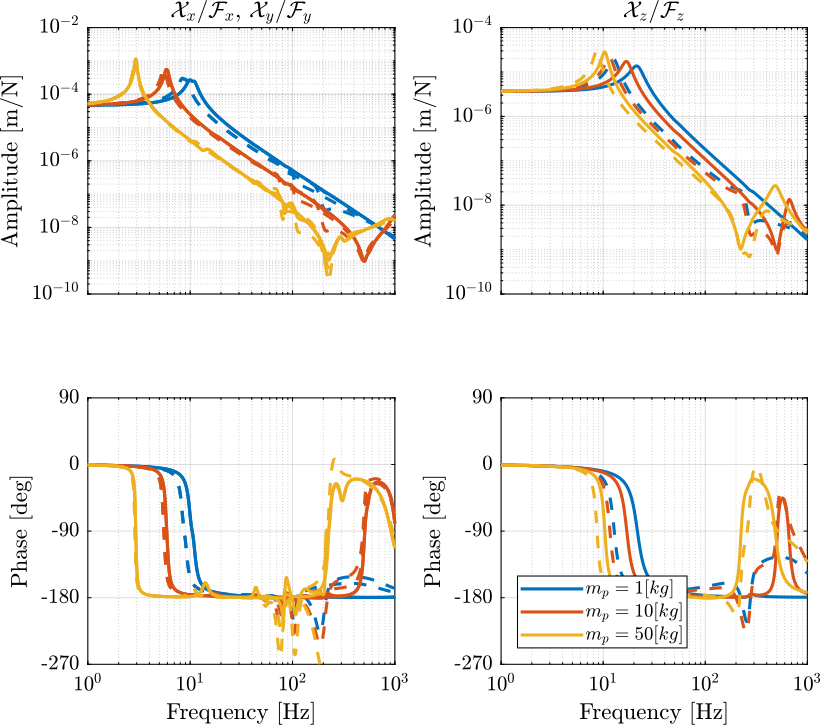
Figure 3: Comparison of the transfer function from \(\mathcal{F}_{x,y,z}\) to \(\mathcal{X}_{x,y,z}\) with and without the virtual addition of mass in the leg’s space
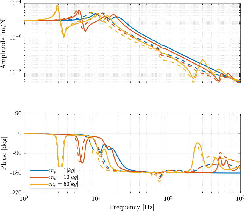
Figure 4: Comparison of the transfer function from \(\tau_i\) to \(\mathcal{L}_{i}\) with and without the virtual addition of mass in the leg’s space
4 Adding Virtual Mass in the Task Space
4.1 Plant
Let’s look at the transfer function from \(\bm{\mathcal{F}}\) to \(d\bm{\mathcal{X}}\): \[ \frac{d\bm{\mathcal{L}}}{\bm{\mathcal{F}}} = \bm{J}^{-1} \frac{d\bm{\mathcal{L}}}{\bm{\tau}} \bm{J}^{-T} \]
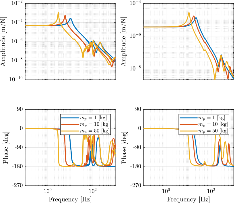
Figure 5: Dynamics from \(\mathcal{F}_{x,y,z}\) to \(\mathcal{X}_{x,y,z}\) used for virtual mass addition in the task space
4.2 Controller Design
KmX = (s^2*1/(1+s/2/pi/500)^2*diag([1 1 50 0 0 0]));
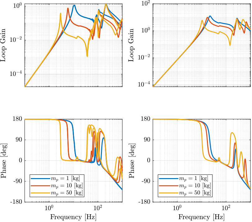
Figure 6: Loop gain for virtual mass addition in the task space
Kdvf = inv(nano_hexapod.kinematics.J')*KmX*inv(nano_hexapod.kinematics.J);
4.3 Identification of the Primary Plant
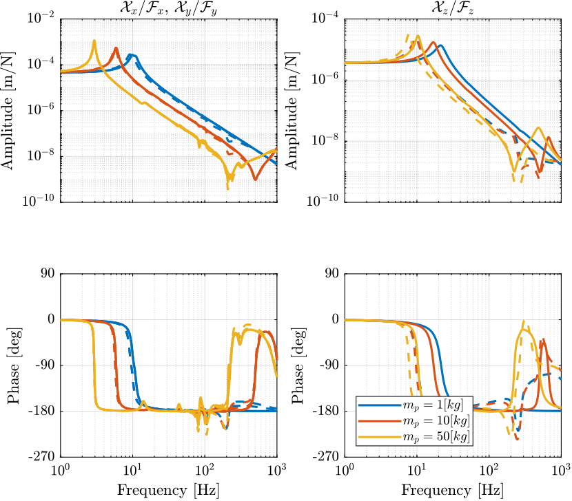
Figure 7: Comparison of the transfer function from \(\mathcal{F}_{x,y,z}\) to \(\mathcal{X}_{x,y,z}\) with and without the virtual addition of mass in the task space
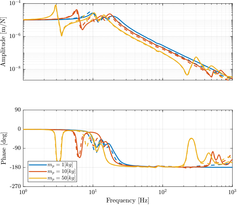
Figure 8: Comparison of the transfer function from \(\tau_i\) to \(\mathcal{L}_{i}\) with and without the virtual addition of mass in the task space