Control Requirements
Table of Contents
- 1. Simplify Model for the Nano-Hexapod
- 2. Control with the Stiff Nano-Hexapod
- 3. Comparison with the use of a Soft nano-hexapod
- 4. Estimate the level of vibration
- 5. Requirements on the norm of closed-loop transfer functions
The goal here is to write clear specifications for the NASS.
This can then be used for the control synthesis and for the design of the nano-hexapod.
Ideal, specifications on the norm of closed loop transfer function should be written.
1 Simplify Model for the Nano-Hexapod
1.1 Model of the nano-hexapod
Let’s consider the simple mechanical system in Figure 1.
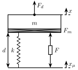
Figure 1: Simplified mechanical system for the nano-hexapod
The signals are described in table 1.
| Symbol | Meaning | |
|---|---|---|
| Exogenous Inputs | \(x_\mu\) | Motion of the $ν$-hexapod’s base |
| \(F_d\) | External Forces applied to the Payload | |
| \(r\) | Reference signal for tracking | |
| Exogenous Outputs | \(x\) | Absolute Motion of the Payload |
| Sensed Outputs | \(F_m\) | Force Sensors in each leg |
| \(d\) | Measured displacement of each leg | |
| \(x\) | Absolute Motion of the Payload | |
| Control Signals | \(F\) | Actuator Inputs |
For the nano-hexapod alone, we have the following equations: \[ \begin{align*} x &= \frac{1}{ms^2 + k} F + \frac{1}{ms^2 + k} F_d + \frac{k}{ms^2 + k} x_\mu \\ F_m &= \frac{ms^2}{ms^2 + k} F - \frac{k}{ms^2 + k} F_d + \frac{k m s^2}{ms^2 + k} x_\mu \\ d &= \frac{1}{ms^2 + k} F + \frac{1}{ms^2 + k} F_d - \frac{ms^2}{ms^2 + k} x_\mu \end{align*} \]
We can write the equations function of \(\omega_\nu = \sqrt{\frac{k}{m}}\): \[ \begin{align*} x &= \frac{1/k}{1 + \frac{s^2}{\omega_\nu^2}} F + \frac{1/k}{1 + \frac{s^2}{\omega_\nu^2}} F_d + \frac{1}{1 + \frac{s^2}{\omega_\nu^2}} x_\mu \\ F_m &= \frac{\frac{s^2}{\omega_\nu^2}}{1 + \frac{s^2}{\omega_\nu^2}} F - \frac{1}{1 + \frac{s^2}{\omega_\nu^2}} F_d + \frac{k \frac{s^2}{\omega_\nu^2}}{1 + \frac{s^2}{\omega_\nu^2}} x_\mu \\ d &= \frac{1/k}{1 + \frac{s^2}{\omega_\nu^2}} F + \frac{1/k}{1 + \frac{s^2}{\omega_\nu^2}} F_d - \frac{\frac{s^2}{\omega_\nu^2}}{1 + \frac{s^2}{\omega_\nu^2}} x_\mu \end{align*} \]
Assumptions:
- the forces applied by the nano-hexapod have no influence on the micro-station, specifically on the displacement of the top platform of the micro-hexapod.
This means that the nano-hexapod can be considered separately from the micro-station and that the motion \(x_\mu\) is imposed and considered as an external input.
The nano-hexapod can thus be represented as in Figure 2.

Figure 2: Block representation of the nano-hexapod
1.2 How to include Ground Motion in the model?
What we measure is not the absolute motion \(x\), but the relative motion \(x - w\) where \(w\) is the motion of the granite.
Also, \(w\) induces some motion \(x_\mu\) through the transmissibility of the micro-station.
1.3 Motion of the micro-station
As explained, we consider \(x_\mu\) as an external input (\(F\) has no influence on \(x_\mu\)).
\(x_\mu\) is the motion of the micro-station’s top platform due to the motion of each stage of the micro-station.
We consider that \(x_\mu\) has the following form: \[ x_\mu = T_\mu r + d_\mu \] where:
- \(T_\mu r\) corresponds to the response of the stages due to the reference \(r\)
- \(d_\mu\) is the motion of the hexapod due to all the vibrations of the stages
\(T_\mu\) can be considered to be a low pass filter with a bandwidth corresponding approximatively to the bandwidth of the micro-station’s stages. To simplify, we can consider \(T_\mu\) to be a first order low pass filter: \[ T_\mu = \frac{1}{1 + s/\omega_\mu} \] where \(\omega_\mu\) corresponds to the tracking speed of the micro-station.
What is important to note is that while \(x_\mu\) is viewed as a perturbation from the nano-hexapod point of view, \(x_\mu\) does depend on the reference signal \(r\).
Also, here, we suppose that the granite is not moving.
If we now include the motion of the granite \(w\), we obtain the block diagram shown in Figure 3.
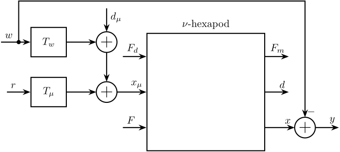
Figure 3: Ground Motion \(w\) included
\(T_w\) is the mechanical transmissibility of the micro-station. We can approximate this transfer function by a second order low pass filter: \[ T_w = \frac{1}{1 + 2 \xi s/\omega_0 + s^2/\omega_0^2} \]
2 Control with the Stiff Nano-Hexapod
2.1 Definition of the values
Let’s define the mass and stiffness of the nano-hexapod.
m = 50; % [kg]
k = 1e7; % [N/m]
Let’s define the Plant as shown in Figure 2:
Gn = 1/(m*s^2 + k)*[-k, k*m*s^2, m*s^2; 1, -m*s^2, 1; 1, k, 1];
Gn.InputName  = {'Fd', 'xmu', 'F'};
Gn.OutputName = {'Fm', 'd', 'x'};
Now, define the transmissibility transfer function \(T_\mu\) corresponding to the micro-station motion.
wmu = 2*pi*50; % [rad/s]

Tmu = 1/(1 + s/wmu);
Tmu.InputName = {'r1'};
Tmu.OutputName = {'ymu'};
w0 = 2*pi*40;
xi = 0.5;
Tw = 1/(1 + 2*xi*s/w0 + s^2/w0^2);
Tw.InputName = {'w1'};
Tw.OutputName = {'dw'};
We add the fact that \(x_\mu = d_\mu + T_\mu r + T_w w\):
Wsplit = [tf(1); tf(1)];
Wsplit.InputName = {'w'};
Wsplit.OutputName = {'w1', 'w2'};

S = sumblk('xmu = ymu + dmu + dw');

Sw = sumblk('y = x - w2');

Gpz = connect(Gn, S, Wsplit, Tw, Tmu, Sw, {'Fd', 'dmu', 'r1', 'F', 'w'}, {'Fm', 'd', 'y'});
2.2 Control using \(d\)
2.2.1 Control Architecture
Let’s consider a feedback loop using \(d\) as shown in Figure 4.
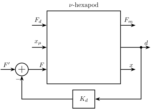
Figure 4: Feedback diagram using \(d\)
2.2.2 Analytical Analysis
Let’s apply a direct velocity feedback by deriving \(d\): \[ F = F^\prime - g s d \]
Thus: \[ d = \frac{1}{ms^2 + gs + k} F^\prime + \frac{1}{ms^2 + gs + k} F_d - \frac{ms^2}{ms^2 + gs + k} x_\mu \]
\[ F = \frac{ms^2 + k}{ms^2 + gs + k} F^\prime - \frac{gs}{ms^2 + gs + k} F_d + \frac{mgs^3}{ms^2 + gs + k} x_\mu \]
and \[ x = \frac{1}{ms^2 + k} (\frac{ms^2 + k}{ms^2 + gs + k} F^\prime - \frac{gs}{ms^2 + gs + k} F_d + \frac{mgs^3}{ms^2 + gs + k} x_\mu) + \frac{1}{ms^2 + k} F_d + \frac{k}{ms^2 + k} x_\mu \]
\[ x = \frac{ms^2 + k}{(ms^2 + k) (ms^2 + gs + k)} F^\prime + \frac{ms^2 + k}{(ms^2 + k) (ms^2 + gs + k)} F_d + \frac{mgs^3 + k(ms^2 + gs + k)}{(ms^2 + k) (ms^2 + gs + k)} x_\mu \]
And we finally obtain: \[ x = \frac{1}{ms^2 + gs + k} F^\prime + \frac{1}{ms^2 + gs + k} F_d + \frac{gs + k}{ms^2 + gs + k} x_\mu \]
K_dvf = 2*sqrt(k*m)*s;
K_dvf.InputName = {'d'};
K_dvf.OutputName = {'F'};

Gpz_dvf = feedback(Gpz, K_dvf, 'name');
Now let’s consider that \(x_\mu = d_\mu + T_\mu r\)
\[ x = \frac{1}{ms^2 + gs + k} F^\prime + \frac{1}{ms^2 + gs + k} F_d + \frac{gs + k}{ms^2 + gs + k} d_\mu + T_\mu \frac{gs + k}{ms^2 + gs + k} r \]
And \(\epsilon = r - x\): \[ \epsilon = \frac{1}{ms^2 + gs + k} F^\prime + \frac{1}{ms^2 + gs + k} F_d + \frac{gs + k}{ms^2 + gs + k} d_\mu + \frac{ms^2 + gs + k - T_\mu (gs + k)}{ms^2 + gs + k} r \]
\[ \epsilon = \frac{1}{ms^2 + gs + k} F^\prime + \frac{1}{ms^2 + gs + k} F_d + \frac{gs + k}{ms^2 + gs + k} d_\mu + \frac{ms^2 - S_\mu(gs + k)}{ms^2 + gs + k} r \]
2.3 Control using \(F_m\)
2.3.1 Control Architecture
Let’s consider a feedback loop using \(Fm\) as shown in Figure 5.
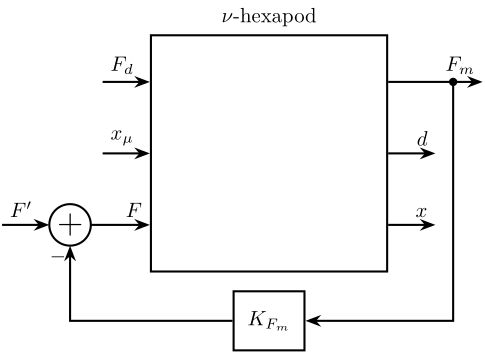
Figure 5: Feedback diagram using \(F_m\)
2.3.2 Pure Integrator
Let’s apply integral force feedback by integration \(F_m\): \[ F = F^\prime - \frac{g}{s} F_m \]
And we finally obtain: \[ x = \frac{1}{ms^2 + mgs + k} F^\prime + \frac{1 + \frac{g}{s}}{ms^2 + mgs + k} F_d + \frac{k}{ms^2 + mgs + k} x_\mu \]
K_iff = 2*sqrt(k/m)/s;
K_iff.InputName = {'Fm'};
K_iff.OutputName = {'F'};

Gpz_iff = feedback(Gpz, K_iff, 'name');
Now let’s consider that \(x_\mu = d_\mu + T_\mu r\)
\[ x = \frac{1}{ms^2 + mgs + k} F^\prime + \frac{1 + \frac{g}{s}}{ms^2 + mgs + k} F_d + \frac{k}{ms^2 + mgs + k} d_\mu + \frac{T_\mu k}{ms^2 + mgs + k} r \]
And \(\epsilon = r - x\): \[ \epsilon = \frac{1}{ms^2 + mgs + k} F^\prime + \frac{1 + \frac{g}{s}}{ms^2 + mgs + k} F_d + \frac{k}{ms^2 + mgs + k} d_\mu + \frac{ms^2 + mgs + k - T_\mu k}{ms^2 + mgs + k} r \]
\[ \epsilon = \frac{1}{ms^2 + mgs + k} F^\prime + \frac{1 + \frac{g}{s}}{ms^2 + mgs + k} F_d + \frac{k}{ms^2 + mgs + k} d_\mu + \frac{ms^2 + mgs + S_\mu k}{ms^2 + mgs + k} r \]
2.3.3 Low pass filter
Instead of a pure integrator, let’s use a low pass filter with a cut-off frequency above the bandwidth of the micro-station \(\omega_mu\)
% K_iff = (2*sqrt(k/m)/(2*wmu))*(1/(1 + s/(2*wmu)));
% K_iff.InputName = {'Fm'};
% K_iff.OutputName = {'F'};

% Gpz_iff = feedback(Gpz, K_iff, 'name');
2.4 Comparison

2.5 Control using \(x\)
2.5.1 Analytical analysis
Let’s first consider that only the output \(x\) is used for feedback (Figure 7)
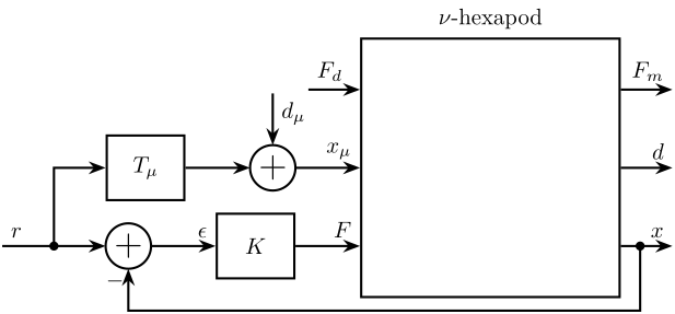
Figure 7: Feedback diagram using \(x\)
We then have: \[ \epsilon &= r - G_{\frac{x}{F}} K \epsilon - G_{\frac{x}{F_d}} F_d - G_{\frac{x}{x_\mu}} d_\mu - G_{\frac{x}{x_\mu}} T_\mu r \]
And then:
\[ \epsilon = \frac{-G_{\frac{x}{F_d}}}{1 + G_{\frac{x}{F}}K} F_d + \frac{-G_{\frac{x}{x_\mu}}}{1 + G_{\frac{x}{F}}K} d_\mu + \frac{1 - G_{\frac{x}{x_\mu}} T_\mu}{1 + G_{\frac{x}{F}}K} r \]
With \(S = \frac{1}{1 + G_{\frac{x}{F}} K}\), we have: \[ \epsilon = - S G_{\frac{x}{F_d}} F_d - S G_{\frac{x}{x_\mu}} d_\mu + S (1 - G_{\frac{x}{x_\mu}} T_\mu) r \]
We have 3 terms that we would like to have small by design:
- \(G_{\frac{x}{F_d}} = \frac{1}{ms^2 + k}\): thus \(k\) and \(m\) should be high to lower the effect of direct forces \(F_d\)
- \(G_{\frac{x}{x_\mu}} = \frac{k}{ms^2 + k} = \frac{1}{1 + \frac{s^2}{\omega_\nu^2}}\): \(\omega_\nu\) should be small enough such that it filters out the vibrations of the micro-station
- \(1 - G_{\frac{x}{x_\mu}} T_\mu\)
\[ 1 - G_{\frac{x}{x_\mu}} T_\mu = 1 - \frac{1}{1 + \frac{s^2}{\omega_\nu^2}} T_\mu \]
We can approximate \(T_\mu \approx \frac{1}{1 + \frac{s}{\omega_\mu}}\) to have:
\begin{align*} 1 - G_{\frac{x}{x_\mu}} T_\mu &= 1 - \frac{1}{1 + \frac{s^2}{\omega_\nu^2}} \frac{1}{1 + \frac{s}{\omega_\mu}} \\ &\approx \frac{\frac{s}{\omega_\mu}}{1 + \frac{s}{\omega_\mu}} = S_\mu \text{ if } \omega_\nu > \omega_\mu \\ &\approx \frac{\frac{s^2}{\omega_\nu^2}}{1 + \frac{s^2}{\omega_\nu^2}} = \text{ if } \omega_\nu < \omega_\mu \end{align*}In our case, we have \(\omega_\nu > \omega_\mu\) and thus we cannot lower this term.
Some implications on the design are summarized on table 2.
| Exogenous Outputs | Design recommendation |
|---|---|
| \(F_d\) | high \(k\), high \(m\) |
| \(d_\mu\) | low \(k\), high \(m\) |
| \(r\) | no influence if \(\omega_\nu > \omega_\mu\) |
2.5.2 Control implementation
Controller for the damped plant using DVF.
wb = 2*pi*50; % control bandwidth [rad/s]

% Lead
h = 2.0;
wz = wb/h; % [rad/s]
wp = wb*h; % [rad/s]

H = 1/h*(1 + s/wz)/(1 + s/wp);

% Integrator until 10Hz
Hi = (1 + s/2/pi/10)/(s/2/pi/10);

K = Hi*H*(1/s);

Kpz_dvf = K/abs(freqresp(K*Gpz_dvf('y', 'F'), wb));
Kpz_dvf.InputName = {'e'};
Kpz_dvf.OutputName = {'Fi'};
Controller for the damped plant using IFF.
wb = 2*pi*50; % control bandwidth [rad/s]

% Lead
h = 2.0;
wz = wb/h; % [rad/s]
wp = wb*h; % [rad/s]

H = 1/h*(1 + s/wz)/(1 + s/wp);

% Integrator until 10Hz
Hi = (1 + s/2/pi/10)/(s/2/pi/10);

K = Hi*H*(1/s);

Kpz_iff = K/abs(freqresp(K*Gpz_iff('y', 'F'), wb));
Kpz_iff.InputName = {'e'};
Kpz_iff.OutputName = {'Fi'};
Loop gain

Let’s connect all the systems as shown in Figure 7.
Sfb = sumblk('e = r2 - y');

R = [tf(1); tf(1)];
R.InputName = {'r'};
R.OutputName = {'r1', 'r2'};

F = [tf(1); tf(1)];
F.InputName = {'Fi'};
F.OutputName = {'F', 'Fu'};

Gpz_fb_dvf = connect(Gpz_dvf, Kpz_dvf, R, Sfb, F, {'r', 'dmu', 'Fd', 'w'}, {'y', 'e', 'Fm', 'd', 'Fu'});
Gpz_fb_iff = connect(Gpz_iff, Kpz_iff, R, Sfb, F, {'r', 'dmu', 'Fd', 'w'}, {'y', 'e', 'Fm', 'd', 'Fu'});
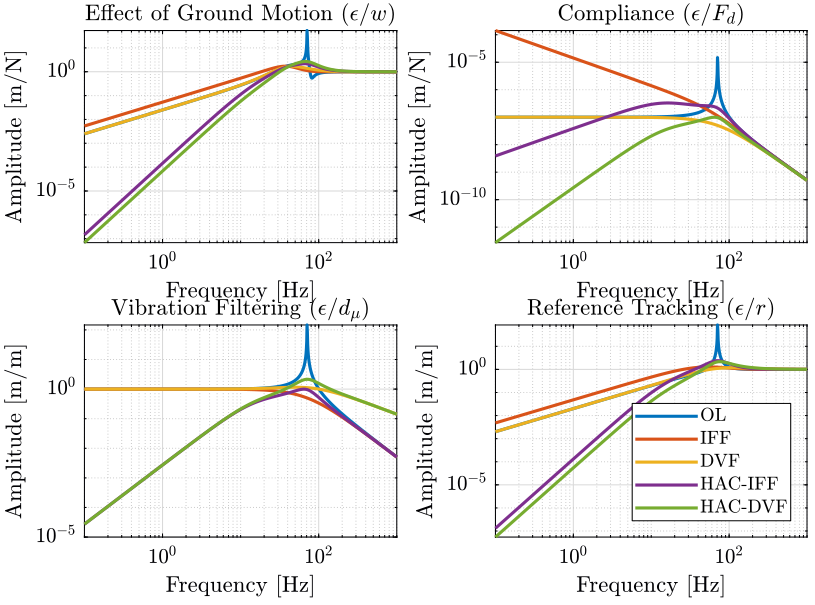
3 Comparison with the use of a Soft nano-hexapod
m = 50; % [kg]
k = 1e3; % [N/m]

Gn = 1/(m*s^2 + k)*[-k, k*m*s^2, m*s^2; 1, -m*s^2, 1; 1, k, 1];
Gn.InputName  = {'Fd', 'xmu', 'F'};
Gn.OutputName = {'Fm', 'd', 'x'};
wmu = 2*pi*50; % [rad/s]

Tmu = 1/(1 + s/wmu);
Tmu.InputName = {'r1'};
Tmu.OutputName = {'ymu'};
w0 = 2*pi*40;
xi = 0.5;
Tw = 1/(1 + 2*xi*s/w0 + s^2/w0^2);
Tw.InputName = {'w1'};
Tw.OutputName = {'dw'};
Wsplit = [tf(1); tf(1)];
Wsplit.InputName = {'w'};
Wsplit.OutputName = {'w1', 'w2'};

S = sumblk('xmu = ymu + dmu + dw');

Sw = sumblk('y = x - w2');

Gvc = connect(Gn, S, Wsplit, Tw, Tmu, Sw, {'Fd', 'dmu', 'r1', 'F', 'w'}, {'Fm', 'd', 'y'});
Kvc_dvf = 2*sqrt(k*m)*s;
Kvc_dvf.InputName = {'d'};
Kvc_dvf.OutputName = {'F'};

Gvc_dvf = feedback(Gvc, Kvc_dvf, 'name');

Kvc_iff = 2*sqrt(k/m)/s;
Kvc_iff.InputName = {'Fm'};
Kvc_iff.OutputName = {'F'};

Gvc_iff = feedback(Gvc, Kvc_iff, 'name');
wb = 2*pi*100; % control bandwidth [rad/s]

% Lead
h = 2.0;
wz = wb/h; % [rad/s]
wp = wb*h; % [rad/s]

H = 1/h*(1 + s/wz)/(1 + s/wp);

Kvc_dvf = H/abs(freqresp(H*Gvc_dvf('y', 'F'), wb));
Kvc_dvf.InputName = {'e'};
Kvc_dvf.OutputName = {'Fi'};

Kvc_iff = H/abs(freqresp(H*Gvc_iff('y', 'F'), wb));
Kvc_iff.InputName = {'e'};
Kvc_iff.OutputName = {'Fi'};
Sfb = sumblk('e = r2 - y');

R = [tf(1); tf(1)];
R.InputName = {'r'};
R.OutputName = {'r1', 'r2'};

F = [tf(1); tf(1)];
F.InputName = {'Fi'};
F.OutputName = {'F', 'Fu'};


Gvc_fb_dvf = connect(Gvc_dvf, Kvc_dvf, R, Sfb, F, {'r', 'dmu', 'Fd', 'w'}, {'y', 'e', 'Fm', 'd', 'Fu'});
Gvc_fb_iff = connect(Gvc_iff, Kvc_iff, R, Sfb, F, {'r', 'dmu', 'Fd', 'w'}, {'y', 'e', 'Fm', 'd', 'Fu'});
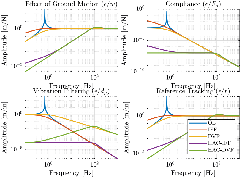
| Reference Tracking | Vibration Filtering | Compliance | |
|---|---|---|---|
| DVF | Similar behavior | Better for \(\omega < \omega_\nu\) | |
| IFF | Similar behavior | Better for \(\omega > \omega_\nu\) |

Figure 11: Comparison of the closed-loop transfer functions for Soft and Stiff nano-hexapod (png, pdf)
| Soft | Stiff | |
|---|---|---|
| Reference Tracking | = | = |
| Ground Motion | = | = |
| Vibration Isolation | + | - |
| Compliance | - | + |
4 Estimate the level of vibration
gm  = load('./mat/psd_gm.mat', 'f', 'psd_gm');
rz  = load('./mat/pxsp_r.mat', 'f', 'pxsp_r');
tyz = load('./mat/pxz_ty_r.mat', 'f', 'pxz_ty_r');
If we note the PSD \(\Gamma\): \[ \Gamma_y = |G_{\frac{y}{w}}|^2 \Gamma_w + |G_{\frac{y}{x_\mu}}|^2 \Gamma_{x_\mu} \]
x_pz = abs(squeeze(freqresp(Gpz_fb_iff('y', 'dmu'), f, 'Hz'))).^2.*(psd_rz + psd_ty) + abs(squeeze(freqresp(Gpz_fb_iff('y', 'w'), f, 'Hz'))).^2.*(psd_gm);
x_vc = abs(squeeze(freqresp(Gvc_fb_iff('y', 'dmu'), f, 'Hz'))).^2.*(psd_rz + psd_ty) + abs(squeeze(freqresp(Gvc_fb_iff('y', 'w'), f, 'Hz'))).^2.*(psd_gm);

Actuator usage
F_pz = abs(squeeze(freqresp(Gpz_fb_iff('Fu', 'dmu'), f, 'Hz'))).^2.*(psd_rz + psd_ty) + abs(squeeze(freqresp(Gpz_fb_iff('Fu', 'w'), f, 'Hz'))).^2.*(psd_gm);
F_vc = abs(squeeze(freqresp(Gvc_fb_iff('Fu', 'dmu'), f, 'Hz'))).^2.*(psd_rz + psd_ty) + abs(squeeze(freqresp(Gvc_fb_iff('Fu', 'w'), f, 'Hz'))).^2.*(psd_gm);
sqrt(trapz(f, F_pz))
sqrt(trapz(f, F_vc))
sqrt(trapz(f, F_pz))
ans =
          84.8961762069446
sqrt(trapz(f, F_vc))
ans =
        0.0387785981815527
5 Requirements on the norm of closed-loop transfer functions
5.1 Approximation of the ASD of perturbations
G_rz = 1e-9*1/(1 + s/2/pi/0.5)^2*(s + 2*pi*1)*(s + 2*pi*10)*(1/((1 + s/2/pi/100)^2));
G_gm = 1e-8*1/s^2*(s + 2*pi*1)^2*(1/((1 + s/2/pi/10)^3));
5.2 Wanted ASD of outputs
Wanted ASD of motion error
y_wanted = 100e-9; % 10nm rms wanted
y_bw = 2*pi*100; % bandwidth [rad/s]

G_y = 2*y_wanted/sqrt(y_bw) * (1 + s/y_bw/10) / (1 + s/y_bw);
sqrt(trapz(f, abs(squeeze(freqresp(G_y, f, 'Hz'))).^2))
sqrt(trapz(f, abs(squeeze(freqresp(G_y, f, 'Hz'))).^2))
ans =
      9.47118350214793e-08
5.3 Limiting the bandwidth
wF = 2*pi*10;
G_F = 100000*(wF + s)^2;
5.4 Generalized Weighted plant
Let’s create a generalized weighted plant for controller synthesis.
Let’s start simple:
| Symbol | Meaning | |
|---|---|---|
| Exogenous Inputs | \(x_\mu\) | Motion of the $ν$-hexapod’s base |
| Exogenous Outputs | \(y\) | Motion error of the Payload |
| Sensed Outputs | \(y\) | Motion error of the Payload |
| Control Signals | \(F\) | Actuator Inputs |
Add \(F\) as output.
F = [tf(1); tf(1)];
F.InputName = {'Fi'};
F.OutputName = {'F', 'Fu'};

P_pz = connect(F, Gpz_dvf, {'dmu', 'Fi'}, {'y', 'Fu', 'y'})
P_vc = connect(F, Gvc_dvf, {'dmu', 'Fi'}, {'y', 'Fu', 'y'})
Normalization.
We multiply the plant input by \(G_{rz}\) and the plant output by \(G_y^{-1}\):
P_pz_norm = blkdiag(inv(G_y), inv(G_F), 1)*P_pz*blkdiag(G_rz, 1);
P_pz_norm.OutputName = {'z', 'F', 'y'};
P_pz_norm.InputName  = {'w', 'u'};

P_vc_norm = blkdiag(inv(G_y), inv(G_F), 1)*P_vc*blkdiag(G_rz, 1);
P_vc_norm.OutputName = {'z', 'F', 'y'};
P_vc_norm.InputName  = {'w', 'u'};
5.5 Synthesis
[Kpz_dvf,CL_vc,~] = hinfsyn(minreal(P_pz_norm), 1, 1, 'TOLGAM', 0.001, 'METHOD', 'LMI', 'DISPLAY', 'on');
Kpz_dvf.InputName = {'e'};
Kpz_dvf.OutputName = {'Fi'};

[Kvc_dvf,CL_pz,~] = hinfsyn(minreal(P_vc_norm), 1, 1, 'TOLGAM', 0.001, 'METHOD', 'LMI', 'DISPLAY', 'on');
Kvc_dvf.InputName = {'e'};
Kvc_dvf.OutputName = {'Fi'};
5.6 Loop Gain
Sfb = sumblk('e = r2 - y');

R = [tf(1); tf(1)];
R.InputName = {'r'};
R.OutputName = {'r1', 'r2'};

F = [tf(1); tf(1)];
F.InputName = {'Fi'};
F.OutputName = {'F', 'Fu'};

Gpz_fb_dvf = connect(Gpz_dvf, -Kpz_dvf, R, Sfb, F, {'r', 'dmu', 'Fd', 'w'}, {'y', 'e', 'Fm', 'd', 'Fu'});
Gvc_fb_dvf = connect(Gvc_dvf, -Kvc_dvf, R, Sfb, F, {'r', 'dmu', 'Fd', 'w'}, {'y', 'e', 'Fm', 'd', 'Fu'});
5.7 Results
5.8 Requirements
| reference tracking | \(\epsilon/r\) | -120dB at 1Hz |
| vibration isolation | \(x/x_\mu\) | -60dB above 10Hz |
| compliance | \(x/F_d\) |