Amplified Piezoelectric Stack Actuator
Table of Contents
The presented model is based on souleille18_concep_activ_mount_space_applic.
The model represents the amplified piezo APA100M from Cedrat-Technologies (Figure 1). The parameters are shown in the table below.
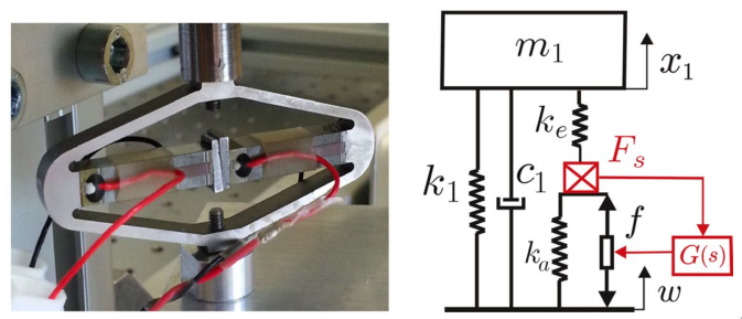
Figure 1: Picture of an APA100M from Cedrat Technologies. Simplified model of a one DoF payload mounted on such isolator
| Value | Meaning | |
|---|---|---|
| \(m\) | \(1\,[kg]\) | Payload mass |
| \(k_e\) | \(4.8\,[N/\mu m]\) | Stiffness used to adjust the pole of the isolator |
| \(k_1\) | \(0.96\,[N/\mu m]\) | Stiffness of the metallic suspension when the stack is removed |
| \(k_a\) | \(65\,[N/\mu m]\) | Stiffness of the actuator |
| \(c_1\) | \(10\,[N/(m/s)]\) | Added viscous damping |
1 Simplified Model
1.1 Parameters
m = 1; % [kg]

ke = 4.8e6; % [N/m]
ce = 5; % [N/(m/s)]
me = 0.001; % [kg]

k1 = 0.96e6; % [N/m]
c1 = 10; % [N/(m/s)]

ka = 65e6; % [N/m]
ca = 5; % [N/(m/s)]
ma = 0.001; % [kg]

h = 0.2; % [m]
IFF Controller:
Kiff = -8000/s;
1.2 Identification
Identification in open-loop.
%% Name of the Simulink File
mdl = 'amplified_piezo_model';

%% Input/Output definition
clear io; io_i = 1;
io(io_i) = linio([mdl, '/w'],  1, 'openinput');  io_i = io_i + 1; % Base Motion
io(io_i) = linio([mdl, '/f'],  1, 'openinput');  io_i = io_i + 1; % Actuator Inputs
io(io_i) = linio([mdl, '/F'],  1, 'openinput');  io_i = io_i + 1; % External Force

io(io_i) = linio([mdl, '/Fs'], 3, 'openoutput'); io_i = io_i + 1; % Force Sensors
io(io_i) = linio([mdl, '/x1'], 1, 'openoutput'); io_i = io_i + 1; % Mass displacement

G = linearize(mdl, io, 0);
G.InputName  = {'w', 'f', 'F'};
G.OutputName = {'Fs', 'x1'};
Identification in closed-loop.
%% Name of the Simulink File
mdl = 'amplified_piezo_model';

%% Input/Output definition
clear io; io_i = 1;
io(io_i) = linio([mdl, '/w'],  1, 'input');  io_i = io_i + 1; % Base Motion
io(io_i) = linio([mdl, '/f'],  1, 'input');  io_i = io_i + 1; % Actuator Inputs
io(io_i) = linio([mdl, '/F'],  1, 'input');  io_i = io_i + 1; % External Force

io(io_i) = linio([mdl, '/Fs'], 3, 'output'); io_i = io_i + 1; % Force Sensors
io(io_i) = linio([mdl, '/x1'], 1, 'output'); io_i = io_i + 1; % Mass displacement

Giff = linearize(mdl, io, 0);
Giff.InputName  = {'w', 'f', 'F'};
Giff.OutputName = {'Fs', 'x1'};
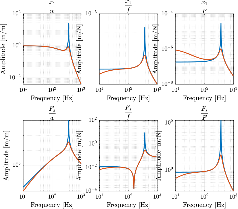
Figure 2: Matrix of transfer functions from input to output in open loop (blue) and closed loop (red)
1.3 Root Locus
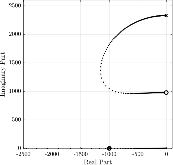
Figure 3: Root Locus
2 Rotating X-Y platform
2.1 Parameters
m = 1; % [kg]

ke = 4.8e6; % [N/m]
ce = 5; % [N/(m/s)]
me = 0.001; % [kg]

k1 = 0.96e6; % [N/m]
c1 = 10; % [N/(m/s)]

ka = 65e6; % [N/m]
ca = 5; % [N/(m/s)]
ma = 0.001; % [kg]

h = 0.2; % [m]
Kiff = tf(0);
2.2 Identification
Rotating speed in rad/s:
Ws = 2*pi*[0, 1, 10, 100];
Gs = {zeros(length(Ws), 1)};
Identification in open-loop.
%% Name of the Simulink File
mdl = 'amplified_piezo_xy_rotating_stage';

%% Input/Output definition
clear io; io_i = 1;
io(io_i) = linio([mdl, '/fx'],  1, 'openinput');  io_i = io_i + 1;
io(io_i) = linio([mdl, '/fy'],  1, 'openinput');  io_i = io_i + 1;

io(io_i) = linio([mdl, '/Fs'], 1, 'openoutput'); io_i = io_i + 1;
io(io_i) = linio([mdl, '/Fs'], 2, 'openoutput'); io_i = io_i + 1;

for i = 1:length(Ws)
    ws = Ws(i);
    G = linearize(mdl, io, 0);
    G.InputName  = {'fx', 'fy'};
    G.OutputName = {'Fsx', 'Fsy'};
    Gs(i) = {G};
end
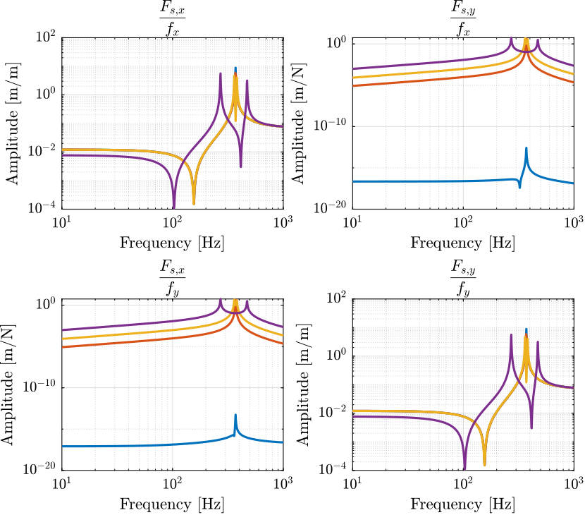
Figure 4: Transfer function matrix from forces to force sensors for multiple rotation speed
2.3 Root Locus
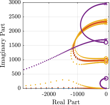
Figure 5: Root locus for 3 rotating speed
2.4 Analysis
The negative stiffness induced by the rotation is equal to \(m \omega_0^2\). Thus, the maximum rotation speed where IFF can be applied is: \[ \omega_\text{max} = \sqrt{\frac{k_1}{m}} \approx 156\,[Hz] \]
Let’s verify that.
Ws = 2*pi*[140, 160];
Identification
%% Name of the Simulink File
mdl = 'amplified_piezo_xy_rotating_stage';

%% Input/Output definition
clear io; io_i = 1;
io(io_i) = linio([mdl, '/fx'],  1, 'openinput');  io_i = io_i + 1;
io(io_i) = linio([mdl, '/fy'],  1, 'openinput');  io_i = io_i + 1;

io(io_i) = linio([mdl, '/Fs'], 1, 'openoutput'); io_i = io_i + 1;
io(io_i) = linio([mdl, '/Fs'], 2, 'openoutput'); io_i = io_i + 1;

for i = 1:length(Ws)
    ws = Ws(i);
    G = linearize(mdl, io, 0);
    G.InputName  = {'fx', 'fy'};
    G.OutputName = {'Fsx', 'Fsy'};
    Gs(i) = {G};
end
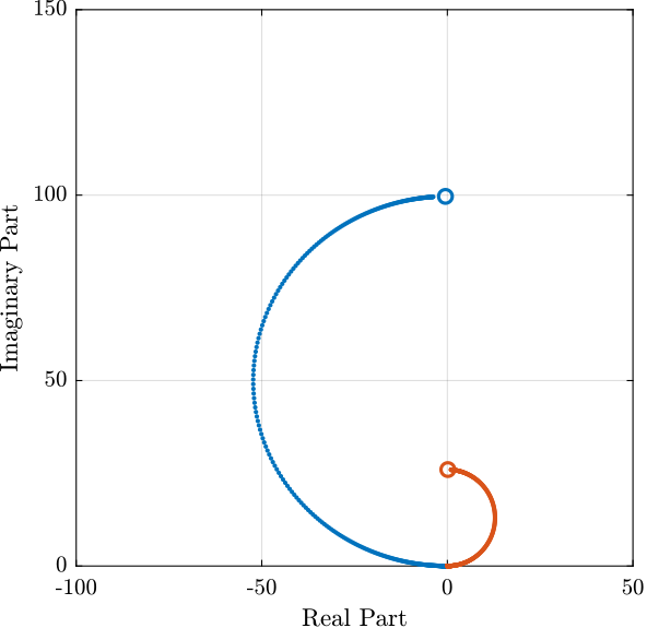
Figure 6: Root Locus for the two considered rotation speed. For the red curve, the system is unstable.