Determination of the optimal nano-hexapod’s stiffness for reducing the effect of disturbances

1. Disturbances
2. Effect of disturbances on the position error
3. Effect of granite stiffness
4. Open Loop Budget Error
5. Closed Loop Budget Error
- 5.1. Reduction thanks to feedback - Required bandwidth
6. Conclusion

In this document is studied how the stiffness of the nano-hexapod will impact the effect of disturbances on the position error of the sample.

It is divided in the following sections:

Section 1: the disturbances are listed and their Power Spectral Densities (PSD) are shown
Section 2: the transfer functions from disturbances to the position error of the sample are computed for a wide range of nano-hexapod stiffnesses
Section 3:
Section 4: from both the PSD of the disturbances and the transfer function from disturbances to sample’s position errors, we compute the resulting PSD and Cumulative Amplitude Spectrum (CAS)
Section 5: from a simplistic model is computed the required control bandwidth to reduce the position error to acceptable values

1 Disturbances

The main disturbances considered here are:

\(D_w\): Ground displacement in the \(x\), \(y\) and \(z\) directions
\(F_{ty}\): Forces applied by the Translation stage in the \(x\) and \(z\) directions
\(F_{rz}\): Forces applied by the Spindle in the \(z\) direction
\(F_d\): Direct forces applied at the center of mass of the Payload

The level of these disturbances has been identified form experiments which are detailed in this document.

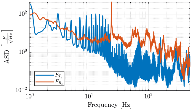
The measured Amplitude Spectral Densities (ASD) of these forces are shown in Figures 1 and 2.

In this study, the expected frequency content of the direct forces applied to the payload is not considered.

Figure 1: Amplitude Spectral Density of the Ground Displacement (png, pdf)

Figure 2: Amplitude Spectral Density of the “parasitic” forces comming from the Translation stage and the spindle (png, pdf)

2 Effect of disturbances on the position error

In this section, we use the Simscape model to identify the transfer function from disturbances to the position error of the sample. We do that for a wide range of nano-hexapod stiffnesses and we compare the obtained results.

2.1 Initialization

We initialize all the stages with the default parameters.

initializeGround();
initializeGranite();
initializeTy();
initializeRy();
initializeRz();
initializeMicroHexapod();
initializeAxisc();
initializeMirror();

We use a sample mass of 10kg.

initializeSample('mass', 10);

We include gravity, and we use no controller.

initializeSimscapeConfiguration('gravity', true);
initializeController();
initializeDisturbances('enable', false);
initializeLoggingConfiguration('log', 'none');

2.2 Identification

The considered inputs are:

Dwx: Ground displacement in the \(x\) direction
Dwy: Ground displacement in the \(y\) direction
Dwz: Ground displacement in the \(z\) direction
Fty_x: Forces applied by the Translation stage in the \(x\) direction
Fty_z: Forces applied by the Translation stage in the \(z\) direction
Frz_z: Forces applied by the Spindle in the \(z\) direction
Fd: Direct forces applied at the center of mass of the Payload

The outputs are Ex, Ey, Ez, Erx, Ery, Erz which are the 3 positions and 3 orientations errors of the sample.

We initialize the set of the nano-hexapod stiffnesses, and for each of them, we identify the dynamics from defined inputs to defined outputs.

Ks = logspace(3,9,7); % [N/m]

2.3 Sensitivity to Stages vibration (Filtering)

The sensitivity the stage vibrations are displayed:

Figure 3: sensitivity to vertical spindle vibrations
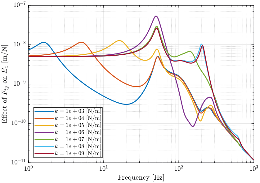
Figure 4: sensitivity to vertical translation stage vibrations
Figure 5: sensitivity to horizontal (x) translation stage vibrations

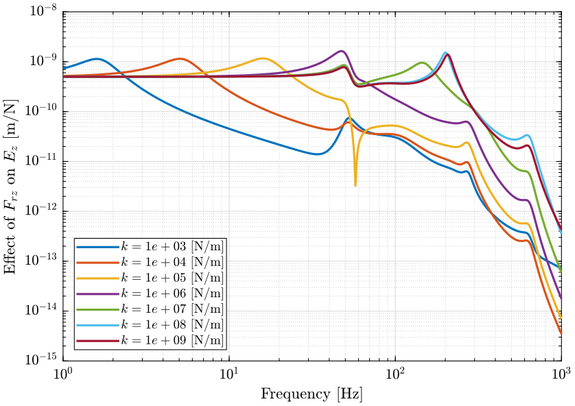
Figure 3: Sensitivity to Spindle vertical motion error (\(F_{rz}\)) to the vertical error position of the sample (\(E_z\)) (png, pdf)

Figure 4: Sensitivity to Translation stage vertical motion error (\(F_{ty,z}\)) to the vertical error position of the sample (\(E_z\)) (png, pdf)

Figure 5: Sensitivity to Translation stage \(x\) motion error (\(F_{ty,x}\)) to the error position of the sample in the \(x\) direction (\(E_x\)) (png, pdf)

2.4 Effect of Ground motion (Transmissibility).

The effect of Ground motion on the position error of the sample is shown in Figure 6.

Figure 6: Sensitivity to Ground motion (\(D_{w}\)) to the position error of the sample (\(E_y\) and \(E_z\)) (png, pdf)

2.5 Direct Forces (Compliance).

The effect of direct forces/torques applied on the sample (cable forces for instance) on the position error of the sample is shown in Figure 7.

Figure 7: Sensitivity to Direct forces and torques applied to the sample (\(F_d\), \(M_d\)) to the position error of the sample (png, pdf)

2.6 Conclusion

Reducing the nano-hexapod stiffness generally lowers the sensitivity to stages vibration but increases the sensitivity to ground motion and direct forces.

In order to conclude on the optimal stiffness that will yield the smallest sample vibration, one has to include the level of disturbances. This is done in Section 4.

3 Effect of granite stiffness

In this section, we wish to see if a soft granite suspension could help in reducing the effect of disturbances on the position error of the sample.

3.1 Analytical Analysis

3.1.1 Simple mass-spring-damper model

Let’s consider the system shown in Figure 8 consisting of two stacked mass-spring-damper systems. The bottom one represents the granite, and the top one all the positioning stages. We want the smallest stage “deformation” \(d = x^\prime - x\) due to ground motion \(w\).

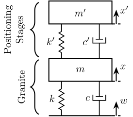
Figure 8: Mass Spring Damper system consisting of a granite and a positioning stage

If we write the equation of motion of the system in Figure 8, we obtain:

\begin{align} m^\prime s^2 x^\prime &= (c^\prime s + k^\prime) (x - x^\prime) \\ ms^2 x &= (c^\prime s + k^\prime) (x^\prime - x) + (cs + k) (w - x) \end{align}

If we note \(d = x^\prime - x\), we obtain:

\begin{equation} \frac{d}{w} = \frac{-m^\prime s^2 (cs + k)}{ (m^\prime s^2 + c^\prime s + k^\prime) (ms^2 + cs + k) + m^\prime s^2(c^\prime s + k^\prime)} \end{equation}

3.1.2 General Case

Let’s now considering a general positioning stage defined by:

\(G^\prime(s) = \frac{F}{x}\): its mechanical “impedance”
\(D^\prime(s) = \frac{d}{x}\): its “deformation” transfer function

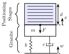
Figure 9: Mass Spring Damper representing the granite and a general representation of positioning stages

The equation of motion are:

\begin{align} ms^2 x &= (cs + k) (x - w) - F \\ F &= G^\prime(s) x \\ d &= D^\prime(s) x \end{align}

where:

\(F\) is the force applied by the position stages on the granite mass

We can express \(d\) as a function of \(w\):

\begin{equation} \frac{d}{w} = \frac{D^\prime(s) (cs + k)}{ms^2 + cs + k + G^\prime(s)} \end{equation}

This is the transfer function that we would like to minimize.

Let’s verify this formula for a simple mass/spring/damper positioning stage. In that case, we have:

\begin{align*} D^\prime(s) &= \frac{d}{x} = \frac{- m^\prime s^2}{m^\prime s^2 + c^\prime s + k^\prime} \\ G^\prime(s) &= \frac{F}{x} = \frac{m^\prime s^2(c^\prime s + k)}{m^\prime s^2 + c^\prime s + k^\prime} \end{align*}

And finally:

\begin{equation} \frac{d}{w} = \frac{-m^\prime s^2 (cs + k)}{ (m^\prime s^2 + c^\prime s + k^\prime) (ms^2 + cs + k) + m^\prime s^2(c^\prime s + k^\prime)} \end{equation}

which is the same as the previously derived equation.

3.2 Soft Granite

Let’s initialize a soft granite and see how the sensitivity to disturbances will change.

initializeGranite('K', 5e5*ones(3,1), 'C', 5e3*ones(3,1));

3.3 Effect of the Granite transfer function

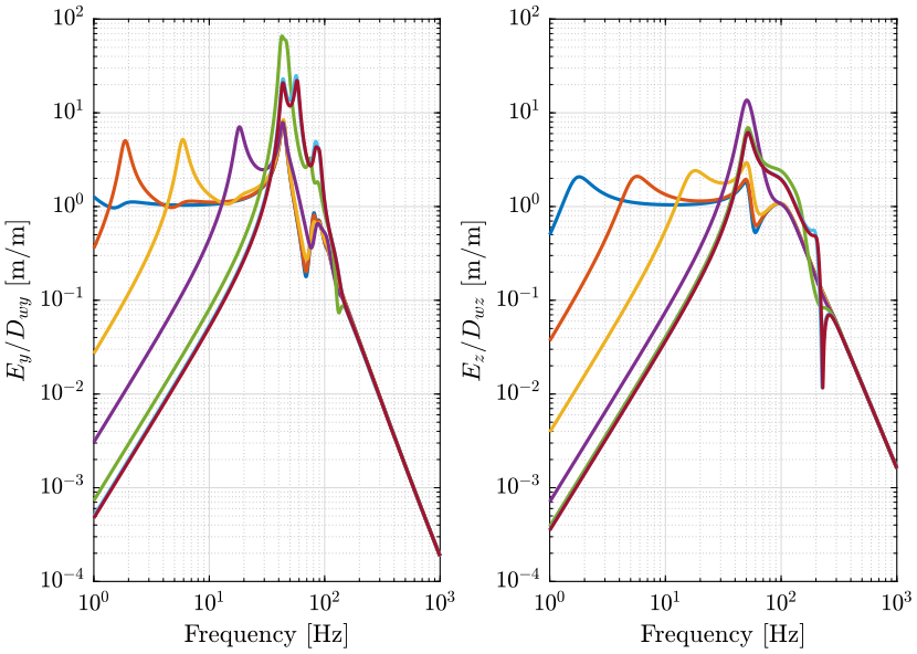
From Figure 10, we can see that having a “soft” granite suspension greatly lowers the sensitivity to ground motion. The sensitivity is indeed lowered starting from the resonance of the granite on its soft suspension (few Hz here).

From Figures 11 and 12, we see that the change of granite suspension does not change a lot the sensitivity to both direct forces and stage vibrations.

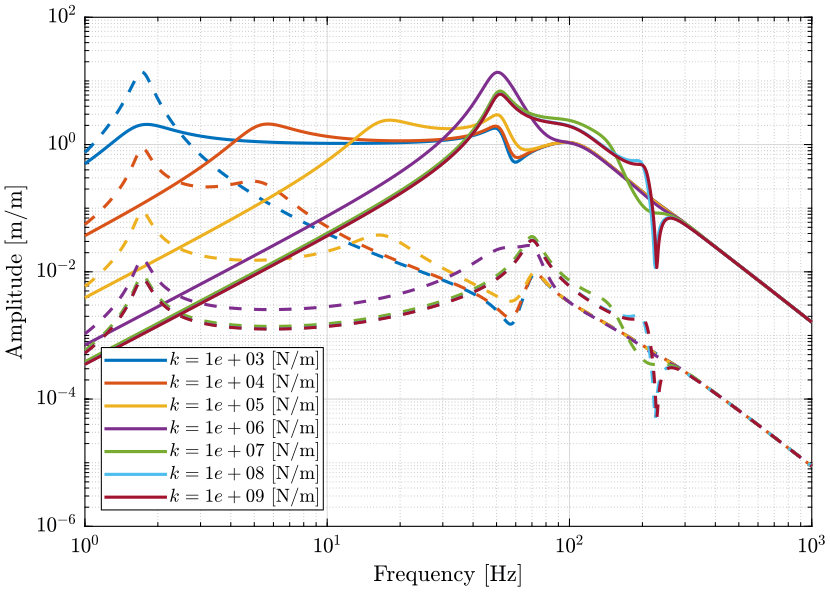
Figure 10: Change of sensibility to Ground motion when using a stiff Granite (solid curves) and a soft Granite (dashed curves) (png, pdf)

Figure 11: Change of sensibility to Spindle vibrations when using a stiff Granite (solid curves) and a soft Granite (dashed curves) (png, pdf)

Figure 12: Change of sensibility to direct forces when using a stiff Granite (solid curves) and a soft Granite (dashed curves) (png, pdf)

3.4 Conclusion

Having a soft granite suspension could greatly improve the sensitivity the ground motion and thus the level of sample vibration if it is found that ground motion is the limiting factor.

4 Open Loop Budget Error

4.1 Load of the identified disturbances and transfer functions

load('./mat/dist_psd.mat', 'dist_f');
load('./mat/opt_stiffness_disturbances.mat', 'Gd')

4.2 Equations

4.3 Results

Effect of all disturbances

freqs = dist_f.f;

figure;
hold on;
for i = 1:length(Ks)
  plot(freqs, sqrt(dist_f.psd_rz).*abs(squeeze(freqresp(Gd{i}('Ez', 'Frz_z'), freqs, 'Hz'))));
end
hold off;
set(gca, 'xscale', 'log'); set(gca, 'yscale', 'log');
xlabel('Frequency [Hz]'); ylabel('ASD $\left[\frac{m}{\sqrt{Hz}}\right]$')
legend('Location', 'southwest');
xlim([2, 500]);

4.4 Cumulative Amplitude Spectrum

freqs = dist_f.f;

figure;
hold on;
for i = 1:length(Ks)
  plot(freqs, sqrt(flip(-cumtrapz(flip(freqs), flip(dist_f.psd_ty.*abs(squeeze(freqresp(Gd{i}('Ez', 'Fty_z'), freqs, 'Hz'))).^2)))), '-', ...
         'DisplayName', sprintf('$k = %.0g$ [N/m]', Ks(i)));
end
plot([freqs(1) freqs(end)], [10e-9 10e-9], 'k--', 'HandleVisibility', 'off');
hold off;
set(gca, 'xscale', 'log'); set(gca, 'yscale', 'log');
xlabel('Frequency [Hz]'); ylabel('CAS $[m]$')
legend('Location', 'southwest');
xlim([2, 500]); ylim([1e-10 1e-6]);

freqs = dist_f.f;

figure;
hold on;
for i = 1:length(Ks)
  plot(freqs, sqrt(flip(-cumtrapz(flip(freqs), flip(dist_f.psd_rz.*abs(squeeze(freqresp(Gd{i}('Ez', 'Frz_z'), freqs, 'Hz'))).^2)))), '-', ...
         'DisplayName', sprintf('$k = %.0g$ [N/m]', Ks(i)));
end
plot([freqs(1) freqs(end)], [10e-9 10e-9], 'k--', 'HandleVisibility', 'off');
hold off;
set(gca, 'xscale', 'log'); set(gca, 'yscale', 'log');
xlabel('Frequency [Hz]'); ylabel('CAS $[m]$')
legend('Location', 'southwest');
xlim([2, 500]); ylim([1e-10 1e-6]);

Ground motion

freqs = dist_f.f;

figure;
hold on;
for i = 1:length(Ks)
  plot(freqs, sqrt(flip(-cumtrapz(flip(freqs), flip(dist_f.psd_gm.*abs(squeeze(freqresp(Gd{i}('Ez', 'Dwz'), freqs, 'Hz'))).^2)))), '-', ...
         'DisplayName', sprintf('$k = %.0g$ [N/m]', Ks(i)));
end
plot([freqs(1) freqs(end)], [10e-9 10e-9], 'k--', 'HandleVisibility', 'off');
hold off;
set(gca, 'xscale', 'log'); set(gca, 'yscale', 'log');
xlabel('Frequency [Hz]'); ylabel('CAS $E_y$ $[m]$')
legend('Location', 'northeast');
xlim([2, 500]); ylim([1e-10 1e-6]);

freqs = dist_f.f;

figure;
hold on;
for i = 1:length(Ks)
  plot(freqs, sqrt(flip(-cumtrapz(flip(freqs), flip(dist_f.psd_gm.*abs(squeeze(freqresp(Gd{i}('Ex', 'Dwx'), freqs, 'Hz'))).^2)))), '-', ...
         'DisplayName', sprintf('$k = %.0g$ [N/m]', Ks(i)));
end
plot([freqs(1) freqs(end)], [10e-9 10e-9], 'k--', 'HandleVisibility', 'off');
hold off;
set(gca, 'xscale', 'log'); set(gca, 'yscale', 'lin');
xlabel('Frequency [Hz]'); ylabel('CAS $E_y$ $[m]$')
legend('Location', 'northeast');
xlim([2, 500]);

freqs = dist_f.f;

figure;
hold on;
for i = 1:length(Ks)
  plot(freqs, sqrt(flip(-cumtrapz(flip(freqs), flip(dist_f.psd_gm.*abs(squeeze(freqresp(Gd{i}('Ey', 'Dwy'), freqs, 'Hz'))).^2)))), '-', ...
         'DisplayName', sprintf('$k = %.0g$ [N/m]', Ks(i)));
end
plot([freqs(1) freqs(end)], [10e-9 10e-9], 'k--', 'HandleVisibility', 'off');
hold off;
set(gca, 'xscale', 'log'); set(gca, 'yscale', 'lin');
xlabel('Frequency [Hz]'); ylabel('CAS $E_y$ $[m]$')
legend('Location', 'northeast');
xlim([2, 500]);

Sum of all perturbations

psd_tot = zeros(length(freqs), length(Ks));

for i = 1:length(Ks)
    psd_tot(:,i) = dist_f.psd_gm.*abs(squeeze(freqresp(Gd{i}('Ez', 'Dwz'  ), freqs, 'Hz'))).^2 + ...
        dist_f.psd_ty.*abs(squeeze(freqresp(Gd{i}('Ez', 'Fty_z'), freqs, 'Hz'))).^2 + ...
        dist_f.psd_rz.*abs(squeeze(freqresp(Gd{i}('Ez', 'Frz_z'), freqs, 'Hz'))).^2;
end

freqs = dist_f.f;

figure;
hold on;
for i = 1:length(Ks)
  plot(freqs, sqrt(flip(-cumtrapz(flip(freqs), flip(psd_tot(:,i))))), '-', ...
         'DisplayName', sprintf('$k = %.0g$ [N/m]', Ks(i)));
end
plot([freqs(1) freqs(end)], [10e-9 10e-9], 'k--', 'HandleVisibility', 'off');
hold off;
set(gca, 'xscale', 'log'); set(gca, 'yscale', 'log');
xlabel('Frequency [Hz]'); ylabel('CAS $E_z$ $[m]$')
legend('Location', 'northeast');
xlim([1, 500]); ylim([1e-10 1e-6]);

5 Closed Loop Budget Error

5.1 Reduction thanks to feedback - Required bandwidth

wc = 1*2*pi; % [rad/s]
xic = 0.5;

S = (s/wc)/(1 + s/wc);

bodeFig({S}, logspace(-1,2,1000))

wc = [1, 5, 10, 20, 50, 100, 200];

S1 = {zeros(length(wc), 1)};
S2 = {zeros(length(wc), 1)};

for j = 1:length(wc)
    L = (2*pi*wc(j))/s; % Simple integrator
    S1{j} = 1/(1 + L);
    L = ((2*pi*wc(j))/s)^2*(1 + s/(2*pi*wc(j)/2))/(1 + s/(2*pi*wc(j)*2));
    S2{j} = 1/(1 + L);
end

freqs = dist_f.f;

figure;
hold on;
i = 6;
for j = 1:length(wc)
    set(gca,'ColorOrderIndex',j);
    plot(freqs, sqrt(flip(-cumtrapz(flip(freqs), flip(abs(squeeze(freqresp(S1{j}, freqs, 'Hz'))).^2.*psd_tot(:,i))))), '-', ...
         'DisplayName', sprintf('$\\omega_c = %.0f$ [Hz]', wc(j)));
end
plot(freqs, sqrt(flip(-cumtrapz(flip(freqs), flip(psd_tot(:,i))))), 'k-', ...
     'DisplayName', 'Open-Loop');
plot([freqs(1) freqs(end)], [10e-9 10e-9], 'k--', 'HandleVisibility', 'off');
hold off;
set(gca, 'xscale', 'log'); set(gca, 'yscale', 'log');
xlabel('Frequency [Hz]'); ylabel('CAS $E_y$ $[m]$')
legend('Location', 'northeast');
xlim([0.5, 500]); ylim([1e-10 1e-6]);

wc = logspace(0, 3, 100);

Dz1_rms = zeros(length(Ks), length(wc));
Dz2_rms = zeros(length(Ks), length(wc));
for i = 1:length(Ks)
    for j = 1:length(wc)
        L = (2*pi*wc(j))/s;
        Dz1_rms(i, j) = sqrt(trapz(freqs, abs(squeeze(freqresp(1/(1 + L), freqs, 'Hz'))).^2.*psd_tot(:,i)));

        L = ((2*pi*wc(j))/s)^2*(1 + s/(2*pi*wc(j)/2))/(1 + s/(2*pi*wc(j)*2));
        Dz2_rms(i, j) = sqrt(trapz(freqs, abs(squeeze(freqresp(1/(1 + L), freqs, 'Hz'))).^2.*psd_tot(:,i)));
    end
end

freqs = dist_f.f;

figure;
hold on;
for i = 1:length(Ks)
  set(gca,'ColorOrderIndex',i);
  plot(wc, Dz1_rms(i, :), '-', ...
         'DisplayName', sprintf('$k = %.0g$ [N/m]', Ks(i)))

  set(gca,'ColorOrderIndex',i);
  plot(wc, Dz2_rms(i, :), '--', ...
         'HandleVisibility', 'off')
end
hold off;
set(gca, 'xscale', 'log'); set(gca, 'yscale', 'log');
xlabel('Control Bandwidth [Hz]'); ylabel('$E_z\ [m, rms]$')
legend('Location', 'southwest');
xlim([1, 500]);