Effect of Uncertainty on the support’s dynamics on the isolation platform dynamics
Table of Contents
- 1. Simple Introductory Example
- 2. Generalization to arbitrary dynamics
In this document we will consider an isolation platform (e.g. the nano-hexapod) on top of a flexible support (e.g. the micro-station).
The goal is to study:
- how does the dynamics of the support influence the dynamics of the plant to control
- similarly: how does the uncertainty on the support’s dynamics will be transferred to uncertainty on the plant
- what design choice should be made in order to minimize the resulting uncertainty on the plant
Two models are made to study these effects:
- In section 1, simple mass-spring-damper systems are chosen to model both the isolation platform and the flexible support
- In section 2, we consider arbitrary support dynamics with multiplicative input uncertainty to study the unmodelled dynamics of the support
1 Simple Introductory Example
Let’s consider the system shown in Figure 1 consisting of:
- A support represented by a mass \(m^\prime\), a stiffness \(k^\prime\) and a dashpot \(c^\prime\)
- An isolation platform represented by a mass \(m\), a stiffness \(k\) and a dashpot \(c\) and an actuator \(F\)
The goal is to stabilize \(x\) using \(F\) in spite of uncertainty on the support mechanical properties.

Figure 1: Two degrees-of-freedom system
1.1 Equations of motion
If we write the equation of motion of the system in Figure 1, we obtain:
\begin{align} ms^2 x &= F + (cs + k) (x^\prime - x) \\ m^\prime s^2 x^\prime &= -F - (c^\prime s + k^\prime) x^\prime + (cs + k)(x - x^\prime) \end{align}After eliminating \(x^\prime\), we obtain:
\begin{equation} \label{org2d73355} \frac{x}{F} = \frac{m^\prime s^2 + c^\prime s + k^\prime}{ms^2(cs + k) + (ms^2 + cs + k)(m^\prime s^2 + c^\prime s + k^\prime)} \end{equation}1.2 Initialization of the support dynamics
Let the support have:
- a nominal mass of \(m^\prime = 1000\ [kg]\)
- a nominal stiffness of \(k^\prime = 10^8\ [N/m]\)
- a nominal damping of \(c^\prime = 10^5\ [N/(m/s)]\)
mpi = 1e3;
cpi = 5e4;
kpi = 1e8;
Let’s also consider some uncertainty in those parameters:
mp = ureal('m', mpi, 'Percentage', 30);
cp = ureal('c', cpi, 'Percentage', 30);
kp = ureal('k', kpi, 'Percentage', 30);
The compliance of the support without the isolation platform is \(\frac{1}{m^\prime s^2 + c^\prime s + k^\prime}\) and its bode plot is shown in Figure 2.
One can see that support has a resonance frequency of \(\omega_0^\prime = 50\ Hz\).

1.3 Initialization of the isolation platform
Let’s first fix the mass of the payload to be isolated:
m = 100;
And we generate three isolation platforms:
- A soft one with \(\omega_0 = 0.1 \omega_0^\prime = 5\ Hz\)
- A medium stiff one with \(\omega_0 = \omega_0^\prime = 50\ Hz\)
- A stiff one with \(\omega_0 = 10 \omega_0^\prime = 500\ Hz\)
1.4 Comparison

1.5 Conclusion
The soft platform dynamics does not seems to depend on the dynamics of the support nor to be affect by the dynamic uncertainty of the support.
2 Generalization to arbitrary dynamics
2.1 Introduction
Let’s now consider a general support described by its compliance \(G^\prime(s) = \frac{x^\prime}{F^\prime}\) as shown in Figure 4.

Figure 4: General support
Now let’s consider the system consisting of a mass-spring-system (the isolation platform) on top of a general support as shown in Figure 5.

Figure 5: Mass-Spring-Damper system on top of a general support
2.2 Equations of motion
We have to following equations of motion:
\begin{align} ms^2 x &= F + (cs + k) (x^\prime - x) \\ F^\prime &= -F + (cs + k)(x - x^\prime) \\ \frac{x^\prime}{F^\prime} &= G^\prime(s) \end{align}And by eliminating \(F^\prime\) and \(x^\prime\), we find the plant dynamics \(G(s) = \frac{x}{F}\).
In order to verify that the formula is correct, let’s take the same mass-spring-damper system used in the system shown in Figure 1: \[ \frac{x^\prime}{F^\prime} = \frac{1}{m^\prime s^2 + c^\prime s + k^\prime} \]
And we obtain \[ \frac{x}{F} = \frac{m^\prime s^2 + c^\prime s + k^\prime}{(ms^2 + cs + k)(m^\prime s^2 + c^\prime s + k^\prime) + ms^2(cs + k)} \] Which is the same transfer function that was obtained in section 1 (Eq. \eqref{eq:plant_simple_system}).
2.3 Compliance of the Support
We model the support by a mass-spring-damper model with some uncertainty.
The nominal compliance of the support is corresponding to the compliance of a mass-spring-damper system with a mass of \(1000\ kg\) and a stiffness of \(10^8\ [N/m]\). The main resonance of the support is then \(\omega^\prime = \sqrt{\frac{m^\prime}{k^\prime}} \approx 50\ Hz\).
m0 = 1e3;
c0 = 5e4;
k0 = 1e8;

Gp0 = 1/(m0*s^2 + c0*s + k0);
Let’s represent the uncertainty on the compliance of the support by a multiplicative uncertainty (Figure 6): \[ G^\prime(s) = G_0^\prime(s)(1 + w_I^\prime(s)\Delta_I(s)) \quad |\Delta_I(j\omega)| < 1\ \forall \omega \]
This could represent unmodelled dynamics or unknown parameters of the support.

Figure 6: Input Multiplicative Uncertainty
We choose a simple uncertainty weight: \[ w_I(s) = \frac{\tau s + r_0}{(\tau/r_\infty) s + 1} \] where \(r_0\) is the relative uncertainty at steady-state, \(1/\tau\) is the frequency at which the relative uncertainty reaches \(100\ \%\), and \(r_\infty\) is the magnitude of the weight at high frequency.
The parameters are defined below.
r0 = 0.5;
tau = 1/(100*2*pi);
rinf = 10;

wI = (tau*s + r0)/((tau/rinf)*s + 1);
We then generate a complex \(\Delta\).
DeltaI = ucomplex('A',0);
We generate the uncertain plant \(G^\prime(s)\).
Gp = Gp0*(1+wI*DeltaI);
A set of uncertainty support’s compliance transfer functions is shown in Figure 7.

2.4 Equivalent Inverse Multiplicative Uncertainty
Let’s express the uncertainty of the plant \(x/F\) as a function of the parameters as well as of the uncertainty on the platform’s compliance:
\begin{align*} \frac{x}{F} &= \frac{1}{ms^2 + cs + k + ms^2(cs + k)G_0^\prime(s)(1 + w_I(s)\Delta(s))}\\ &= \frac{1}{ms^2 + cs + k + ms^2(cs + k)G_0^\prime(s) + ms^2(cs + k)G_0^\prime(s) w_I(s)\Delta(s)}\\ &= \frac{1}{ms^2 + cs + k + ms^2(cs + k)G_0^\prime(s)} \cdot \frac{1}{1 + \frac{ms^2(cs + k)G_0^\prime(s) w_I(s)}{ms^2 + cs + k + ms^2(cs + k)G_0^\prime(s)} \Delta(s)}\\ \end{align*}We can the plant dynamics that as an inverse multiplicative uncertainty (Figure 8):
\begin{equation} \frac{x}{F} = G_0(s) (1 + w_{iI}(s) \Delta(s))^{-1} \end{equation}with:
- \(G_0(s) = \frac{1}{ms^2 + cs + k + ms^2(cs + k)G_0^\prime(s)}\)
- \(w_{iI}(s) = \frac{ms^2(cs + k)G_0^\prime(s) w_I(s)}{ms^2 + cs + k + ms^2(cs + k)G_0^\prime(s)} = G_0(s) ms^2(cs + k)G_0^\prime(s) w_I(s)\)

Figure 8: Inverse Multiplicative Uncertainty
2.5 Effect of the Isolation platform Stiffness
Let’s first fix the mass of the payload to be isolated:
m = 100;
And we generate three isolation platforms:
- A soft one with \(\omega_0 = 5\ Hz\)
- A medium stiff one with \(\omega_0 = 50\ Hz\)
- A stiff one with \(\omega_0 = 500\ Hz\)
Soft Isolation Platform:
k_soft = m*(2*pi*5)^2;
c_soft = 0.1*sqrt(m*k_soft);

G_soft = 1/(m*s^2 + c_soft*s + k_soft + m*s^2*(c_soft*s + k_soft)*Gp);
G0_soft = 1/(m*s^2 + c_soft*s + k_soft + m*s^2*(c_soft*s + k_soft)*Gp0);
wiI_soft = Gp0*m*s^2*(c_soft*s + k_soft)*G0_soft*wI;
Mid Isolation Platform
k_mid = m*(2*pi*50)^2;
c_mid = 0.1*sqrt(m*k_mid);

G_mid = 1/(m*s^2 + c_mid*s + k_mid + m*s^2*(c_mid*s + k_mid)*Gp);
G0_mid = 1/(m*s^2 + c_mid*s + k_mid + m*s^2*(c_mid*s + k_mid)*Gp0);
wiI_mid = Gp0*m*s^2*(c_mid*s + k_mid)*G0_mid*wI;
Stiff Isolation Platform
k_stiff = m*(2*pi*500)^2;
c_stiff = 0.1*sqrt(m*k_stiff);

G_stiff = 1/(m*s^2 + c_stiff*s + k_stiff + m*s^2*(c_stiff*s + k_stiff)*Gp);
G0_stiff = 1/(m*s^2 + c_stiff*s + k_stiff + m*s^2*(c_stiff*s + k_stiff)*Gp0);
wiI_stiff = Gp0*m*s^2*(c_stiff*s + k_stiff)*G0_stiff*wI;
The obtained transfer functions \(x/F\) for each of the three platforms are shown in Figure 9.

The obtain result is very similar to the one obtain in section 1, except for the stiff isolation that experience lot’s of uncertainty at high frequency. This is due to the fact that with the current model, at high frequency, the support’s compliance uncertainty is much higher than the previous model.
2.6 Reduce the Uncertainty on the plant
Now that we know the expression of the uncertainty on the plant, we can wonder what parameters of the isolation platform would lower the plant uncertainty, or at least bring the uncertainty to reasonable level.
The uncertainty of the plant is described by an inverse multiplicative uncertainty with the following weight: \[ w_{iI}(s) = \frac{ms^2(cs + k)G_0^\prime(s) w_I(s)}{ms^2 + cs + k + ms^2(cs + k)G_0^\prime(s)} \]
Let’s study separately the effect of the platform’s mass, damping and stiffness.
2.6.1 Effect of the platform’s stiffness \(k\)
Let’s fix \(\xi = \frac{c}{2\sqrt{km}} = 0.1\), \(m = 100\ [kg]\) and see the evolution of \(|w_{iI}(j\omega)|\) with \(k\).
This is first shown for few values of the stiffness \(k\) in figure 10

The norm of the uncertainty weight \(|w_iI(j\omega)|\) is displayed as a function of \(\omega\) and \(k\) in Figure 11.
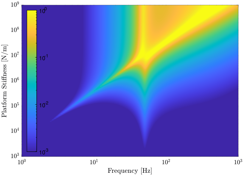
Figure 11: Evolution of the norm of the uncertainty weight \(|w_{iI}(j\omega)|\) as a function of the platform’s stiffness \(k\) (png, pdf)
Instead of plotting as a function of the platform’s stiffness, we can plot as a function of \(\omega_0/\omega_0^\prime\) where:
- \(\omega_0\) is the resonance of the platform alone
- \(\omega_0^\prime\) is the resonance of the support alone
The obtain plot is shown in Figure 12. In that case, we can see that with a platform’s resonance frequency 10 times lower than the resonance of the support, we get less than \(1\%\) uncertainty.

2.6.2 Effect of the platform’s damping \(c\)

2.6.3 Effect of the platform’s mass \(m\)

2.7 Conclusion
If the goal is to have an acceptable (\(<10\%\)) uncertainty on the plant until the highest frequency, two design choice for the isolation platform are possible:
- a very soft isolation platform \(\omega_0 \ll \omega_0^\prime\)
- a very stiff isolation platform \(\omega_0 \gg \omega_0^\prime\)
If a very soft isolation platform is used, the uncertainty due to the support’s compliance is filtered out and never reaches problematic values.
If a very stiff isolation platform is used, the uncertainty will be high around \(\omega_0^\prime\) and may reach unacceptable value. It will then be high around \(\omega_0\) and probably be higher than one. Thus, if a stiff isolation platform is used, the recommendation is to have the largest possible resonance frequency, as the control bandwidth will be limited by the first resonance of the isolation platform (if not already limited by the resonance of the support).