Study of the Flexible Joints

1. Bending and Torsional Stiffness
2. Axial Stiffness
3. Conclusion

In this document is studied the effect of the mechanical behavior of the flexible joints that are located the extremities of each nano-hexapod’s legs.

Ideally, we want the x and y rotations to be free and all the translations to be blocked. However, this is never the case and be have to consider:

Finite bending stiffnesses (Section 1)
Axial stiffness in the direction of the legs (Section 2)

This may impose some limitations, also, the goal is to specify the required joints stiffnesses (summarized in Section 3).

1 Bending and Torsional Stiffness

In this section, we wish to study the effect of the rotation flexibility of the nano-hexapod joints.

1.1 Initialization

Let’s initialize all the stages with default parameters.

initializeGround();
initializeGranite();
initializeTy();
initializeRy();
initializeRz();
initializeMicroHexapod();
initializeAxisc();
initializeMirror();

Let’s consider the heaviest mass which should we the most problematic with it comes to the flexible joints.

initializeSample('mass', 50, 'freq', 200*ones(6,1));
initializeReferences('Rz_type', 'rotating-not-filtered', 'Rz_period', 60);

1.2 Realistic Bending Stiffness Values

Let’s compare the ideal case (zero stiffness in rotation and infinite stiffness in translation) with a more realistic case:

\(K_{\theta, \phi} = 15\,[Nm/rad]\) stiffness in flexion
\(K_{\psi} = 20\,[Nm/rad]\) stiffness in torsion

Kf_M = 15*ones(6,1);
Kf_F = 15*ones(6,1);
Kt_M = 20*ones(6,1);
Kt_F = 20*ones(6,1);

The stiffness and damping of the nano-hexapod’s legs are:

k_opt = 1e5; % [N/m]
c_opt = 2e2; % [N/(m/s)]

This corresponds to the optimal identified stiffness.

1.2.1 Direct Velocity Feedback

We identify the dynamics from actuators force \(\tau_i\) to relative motion sensors \(d\mathcal{L}_i\) with and without considering the flexible joint stiffness.

The obtained dynamics are shown in Figure 1. It is shown that the adding of stiffness for the flexible joints does increase a little bit the frequencies of the mass suspension modes. It stiffen the structure.

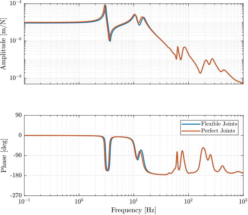
Figure 1: Dynamics from actuators force \(\tau_i\) to relative motion sensors \(d\mathcal{L}_i\) with (blue) and without (red) considering the flexible joint stiffness

1.2.2 Primary Plant

Let’s now identify the dynamics from \(\bm{\tau}^\prime\) to \(\bm{\epsilon}_{\mathcal{X}_n}\) (for the primary controller designed in the frame of the legs).

The dynamics is compare with and without the joint flexibility in Figure 2. The plant dynamics is not found to be changing significantly.

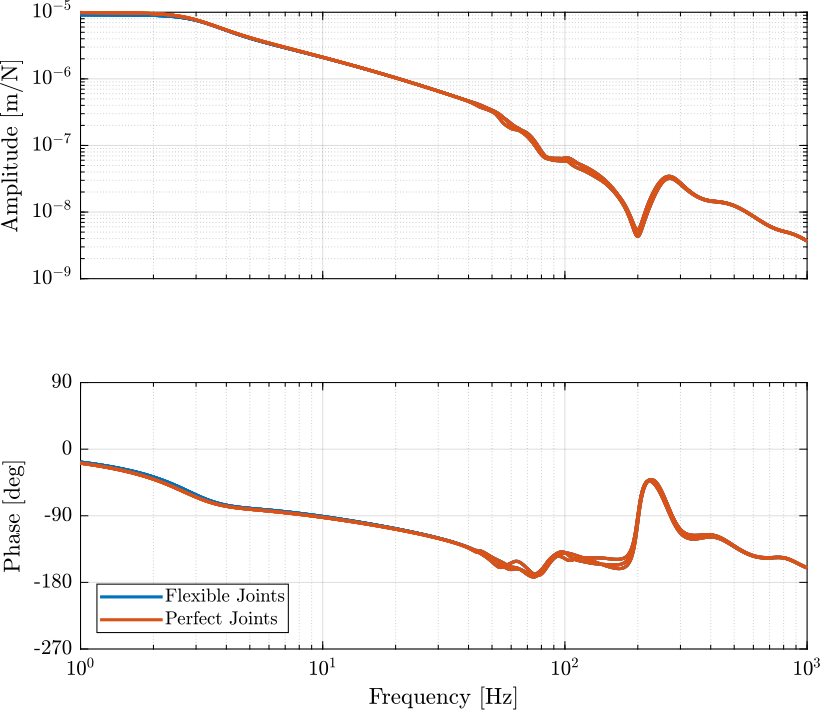
Figure 2: Dynamics from \(\bm{\tau}^\prime_i\) to \(\bm{\epsilon}_{\mathcal{X}_n,i}\) with perfect joints and with flexible joints

1.2.3 Conclusion

Considering realistic flexible joint bending stiffness for the nano-hexapod does not seems to impose any limitation on the DVF control nor on the primary control.

It only increases a little bit the suspension modes of the sample on top of the nano-hexapod.

1.3 Parametric Study

We wish now to see what is the impact of the rotation stiffness of the flexible joints on the dynamics. This will help to determine the requirements on the joint’s stiffness.

Let’s consider the following bending stiffness of the flexible joints:

Ks = [1, 5, 10, 50, 100]; % [Nm/rad]

We also consider here a nano-hexapod with the identified optimal actuator stiffness.

1.3.1 Direct Velocity Feedback

The dynamics from the actuators to the relative displacement sensor in each leg is identified and shown in Figure 3.

The corresponding Root Locus plot is shown in Figure 4.

It is shown that the bending stiffness of the flexible joints does indeed change a little the dynamics, but critical damping is stiff achievable with Direct Velocity Feedback.

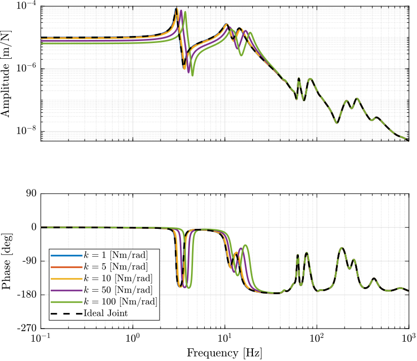
Figure 3: Dynamics from \(\tau_i\) to \(d\mathcal{L}_i\) for all the considered Rotation Stiffnesses

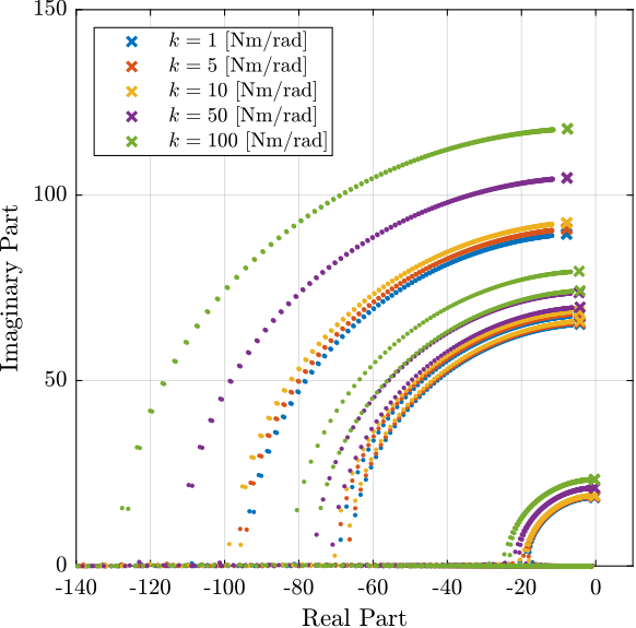
Figure 4: Root Locus for all the considered Rotation Stiffnesses

1.3.2 Primary Control

The dynamics from \(\bm{\tau}^\prime\) to \(\bm{\epsilon}_{\mathcal{X}_n}\) (for the primary controller designed in the frame of the legs) is shown in Figure 5.

It is shown that the bending stiffness of the flexible joints have very little impact on the dynamics.

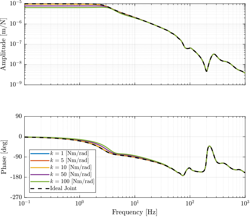
Figure 5: Diagonal elements of the transfer function matrix from \(\bm{\tau}^\prime\) to \(\bm{\epsilon}_{\mathcal{X}_n}\) for the considered bending stiffnesses

1.3.3 Conclusion

The bending stiffness of the flexible joint does not significantly change the dynamics.

2 Axial Stiffness

Let’s know consider a flexibility in translation of the flexible joint, in the axis of the legs.

2.1 Realistic Translation Stiffness Values

We choose realistic values of the axial stiffness of the joints: \[ K_a = 60\,[N/\mu m] \]

Kz_F = 60e6*ones(6,1); % [N/m]
Kz_M = 60e6*ones(6,1); % [N/m]
Cz_F = 1*ones(6,1); % [N/(m/s)]
Cz_M = 1*ones(6,1); % [N/(m/s)]

2.1.1 Initialization

Let’s initialize all the stages with default parameters.

initializeGround();
initializeGranite();
initializeTy();
initializeRy();
initializeRz();
initializeMicroHexapod();
initializeAxisc();
initializeMirror();

Let’s consider the heaviest mass which should we the most problematic with it comes to the flexible joints.

initializeSample('mass', 50, 'freq', 200*ones(6,1));
initializeReferences('Rz_type', 'rotating-not-filtered', 'Rz_period', 60);

2.1.2 Direct Velocity Feedback

The dynamics from actuators force \(\tau_i\) to relative motion sensors \(d\mathcal{L}_i\) with and without considering the flexible joint stiffness are identified.

The obtained dynamics are shown in Figure 6.

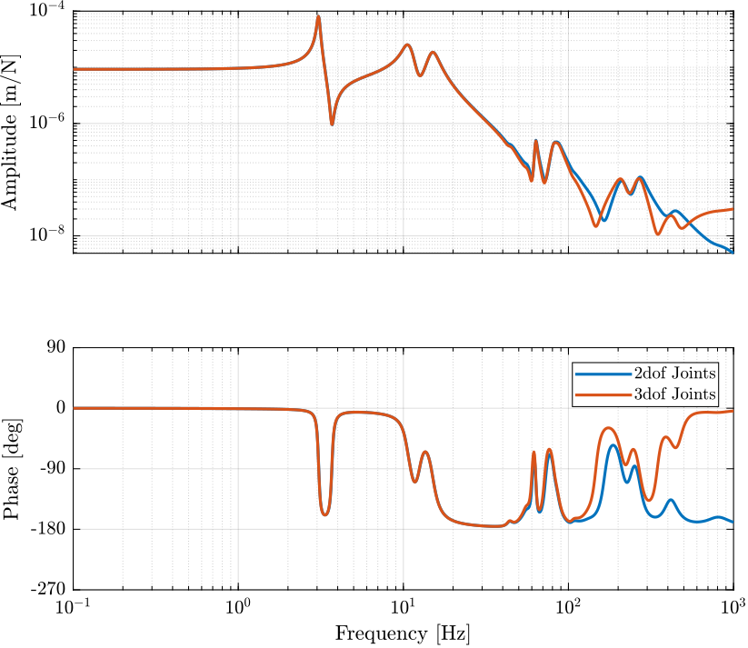
Figure 6: Dynamics from actuators force \(\tau_i\) to relative motion sensors \(d\mathcal{L}_i\) with (blue) and without (red) considering the flexible joint axis stiffness

2.1.3 Primary Plant

Kdvf = 5e3*s/(1+s/2/pi/1e3)*eye(6);

Let’s now identify the dynamics from \(\bm{\tau}^\prime\) to \(\bm{\epsilon}_{\mathcal{X}_n}\) (for the primary controller designed in the frame of the legs).

The dynamics is compare with and without the joint flexibility in Figure 7.

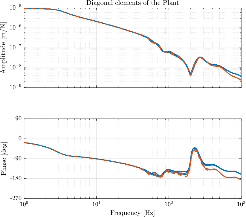
Figure 7: Dynamics from \(\bm{\tau}^\prime_i\) to \(\bm{\epsilon}_{\mathcal{X}_n,i}\) with infinite axis stiffnes (solid) and with realistic axial stiffness (dashed)

2.1.4 Conclusion

For the realistic value of the flexible joint axial stiffness, the dynamics is not much impact, and this should not be a problem for control.

2.2 Parametric study

We wish now to see what is the impact of the axial stiffness of the flexible joints on the dynamics.

Let’s consider the following values for the axial stiffness:

Kzs = [1e4, 1e5, 1e6, 1e7, 1e8, 1e9]; % [N/m]

We also consider here a nano-hexapod with the identified optimal actuator stiffness (\(k = 10^5\,[N/m]\)).

2.2.1 Direct Velocity Feedback

The dynamics from the actuators to the relative displacement sensor in each leg is identified and shown in Figure 8.

It is shown that the axial stiffness of the flexible joints does have a huge impact on the dynamics.

If the axial stiffness of the flexible joints is \(K_a > 10^7\,[N/m]\) (here \(100\) times higher than the actuator stiffness), then the change of dynamics stays reasonably small.

This is more clear by looking at the root locus (Figures 9 and 10). It can be seen that very little active damping can be achieve for axial stiffnesses below \(10^7\,[N/m]\).

Figure 8: Dynamics from \(\tau_i\) to \(d\mathcal{L}_i\) for all the considered axis Stiffnesses

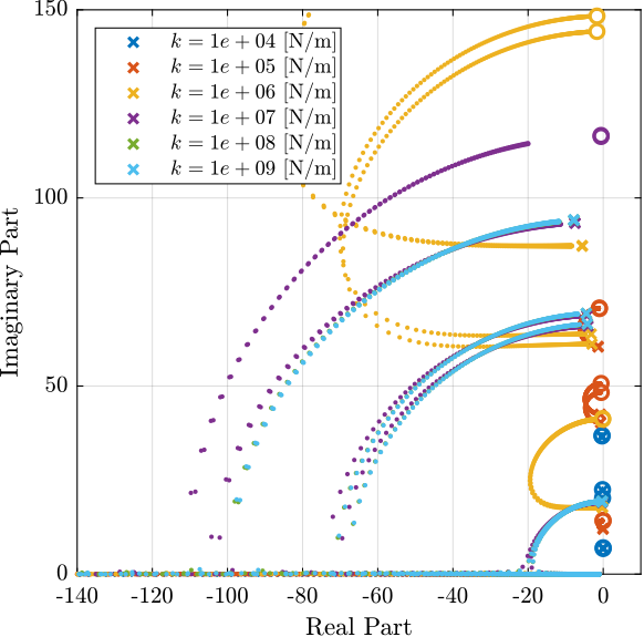
Figure 9: Root Locus for all the considered axial Stiffnesses

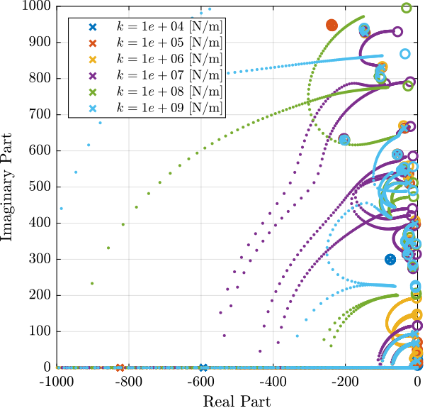
Figure 10: Root Locus (unzoom) for all the considered axial Stiffnesses

2.2.2 Primary Control

The dynamics from \(\bm{\tau}^\prime\) to \(\bm{\epsilon}_{\mathcal{X}_n}\) (for the primary controller designed in the frame of the legs) is shown in Figure 11.

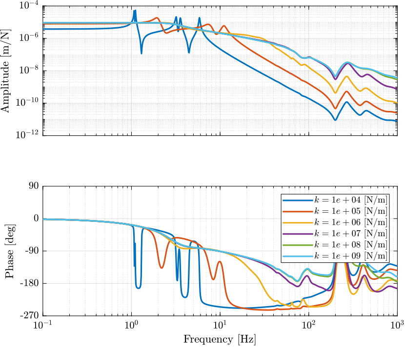
Figure 11: Diagonal elements of the transfer function matrix from \(\bm{\tau}^\prime\) to \(\bm{\epsilon}_{\mathcal{X}_n}\) for the considered axial stiffnesses

2.3 Conclusion

The axial stiffness of the flexible joints should be maximized.

For the considered actuator stiffness \(k = 10^5\,[N/m]\), the axial stiffness of the flexible joints should ideally be above \(10^7\,[N/m]\).

This is a reasonable stiffness value for such joints.

We may interpolate the results and say that the axial joint stiffness should be 100 times higher than the actuator stiffness, but this should be confirmed with further analysis.

3 Conclusion

In this study we considered the bending, torsional and axial stiffnesses of the flexible joints used for the nano-hexapod.

The bending and torsional stiffnesses somehow adds a parasitic stiffness in parallel with the legs. It is not found to be much problematic for the considered control architecture (it is however, if Integral Force Feedback is to be used). As a consequence of the added stiffness, it could increase a little bit the required actuator force.

The axial stiffness of the flexible joints can be very problematic for control. Small values of the axial stiffness are shown to limit the achievable damping with Direct Velocity Feedback. The axial stiffness should therefore be maximized and taken into account in the model of the nano-hexapod.

For the identified optimal actuator stiffness \(k = 10^5\,[N/m]\), the flexible joint should have the following stiffness properties:

Axial Stiffness: \(K_a > 10^7\,[N/m]\)
Bending Stiffness: \(K_b < 50\,[Nm/rad]\)
Torsion Stiffness: \(K_t < 50\,[Nm/rad]\)

As there is generally a trade-off between bending stiffness and axial stiffness, it should be highlighted that the axial stiffness is the most important property of the flexible joints.