Control of the NASS with optimal stiffness
Table of Contents
1 Low Authority Control - Decentralized Direct Velocity Feedback
1.1 Initialization
initializeGround();
initializeGranite();
initializeTy();
initializeRy();
initializeRz();
initializeMicroHexapod();
initializeAxisc();
initializeMirror();

initializeSimscapeConfiguration();
initializeDisturbances('enable', false);
initializeLoggingConfiguration('log', 'none');

initializeController('type', 'hac-dvf');
We set the stiffness of the payload fixation:
Kp = 1e8; % [N/m]
1.2 Identification
K = tf(zeros(6));
Kdvf = tf(zeros(6));
We identify the system for the following payload masses:
Ms = [1, 10, 50];
The nano-hexapod has the following leg’s stiffness and damping.
initializeNanoHexapod('k', 1e5, 'c', 2e2);
1.3 Controller Design
The obtain dynamics from actuators forces \(\tau_i\) to the relative motion of the legs \(d\mathcal{L}_i\) is shown in Figure 2 for the three considered payload masses.
The Root Locus is shown in Figure 3 and wee see that we have unconditional stability.
In order to choose the gain such that we obtain good damping for all the three payload masses, we plot the damping ration of the modes as a function of the gain for all three payload masses in Figure 4.
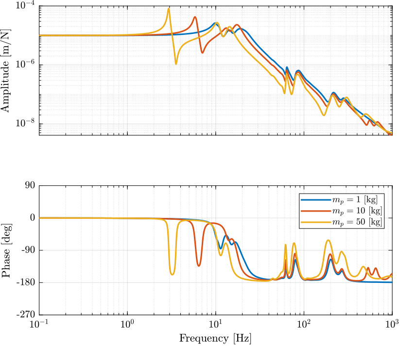
Figure 2: Dynamics for the Direct Velocity Feedback active damping for three payload masses
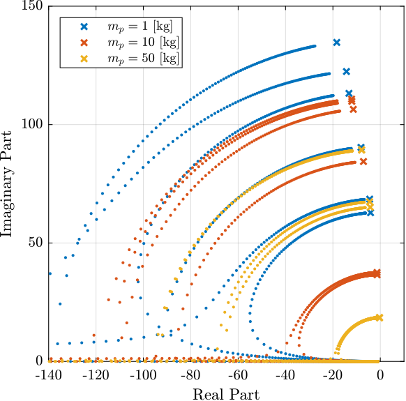
Figure 3: Root Locus for the DVF controll for three payload masses
Damping as function of the gain
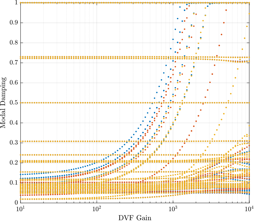
Figure 4: Damping ratio of the poles as a function of the DVF gain
Finally, we use the following controller for the Decentralized Direct Velocity Feedback:
Kdvf = 5e3*s/(1+s/2/pi/1e3)*eye(6);
1.4 Effect of the Low Authority Control on the Primary Plant
Let’s identify the dynamics from actuator forces \(\bm{\tau}\) to displacement as measured by the metrology \(\bm{\mathcal{X}}\): \[ \bm{G}(s) = \frac{\bm{\mathcal{X}}}{\bm{\tau}} \] We do so both when the DVF is applied and when it is not applied.
Then, we compute the transfer function from forces applied by the actuators \(\bm{\mathcal{F}}\) to the measured position error in the frame of the nano-hexapod \(\bm{\epsilon}_{\mathcal{X}_n}\): \[ \bm{G}_\mathcal{X}(s) = \frac{\bm{\epsilon}_{\mathcal{X}_n}}{\bm{\mathcal{F}}} = \bm{G}(s) \bm{J}^{-T} \] The obtained dynamics is shown in Figure 5.
A zero with a positive real part is introduced in the transfer function from \(\mathcal{F}_y\) to \(\mathcal{X}_y\) after Decentralized Direct Velocity Feedback is applied.
And we compute the transfer function from actuator forces \(\bm{\tau}\) to position error of each leg \(\bm{\epsilon}_\mathcal{L}\): \[ \bm{G}_\mathcal{L} = \frac{\bm{\epsilon}_\mathcal{L}}{\bm{\tau}} = \bm{J} \bm{G}(s) \] The obtained dynamics is shown in Figure 6.
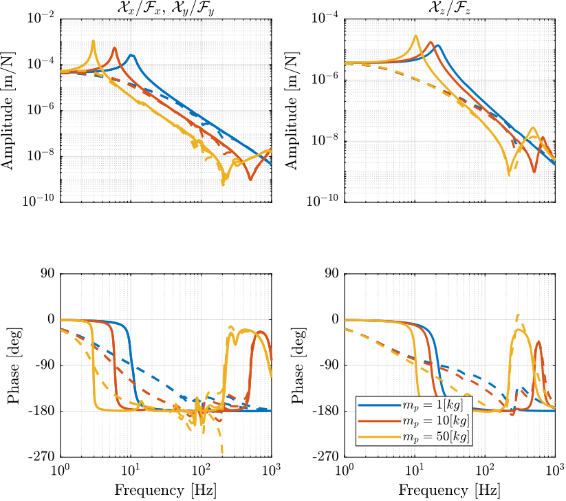
Figure 5: Primary plant in the task space with (dashed) and without (solid) Direct Velocity Feedback
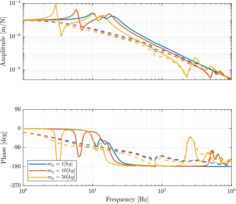
Figure 6: Primary plant in the space of the legs with (dashed) and without (solid) Direct Velocity Feedback
The coupling (off diagonal elements) of \(\bm{G}_\mathcal{X}\) are shown in Figure 7 both when DVF is applied and when it is not.
The coupling does not change a lot with DVF.
The coupling in the space of the legs \(\bm{G}_\mathcal{L}\) are shown in Figure 8.
The magnitude of the coupling between \(\tau_i\) and \(d\mathcal{L}_j\) (Figure 8) around the resonance of the nano-hexapod (where the coupling is the highest) is considerably reduced when DVF is applied.
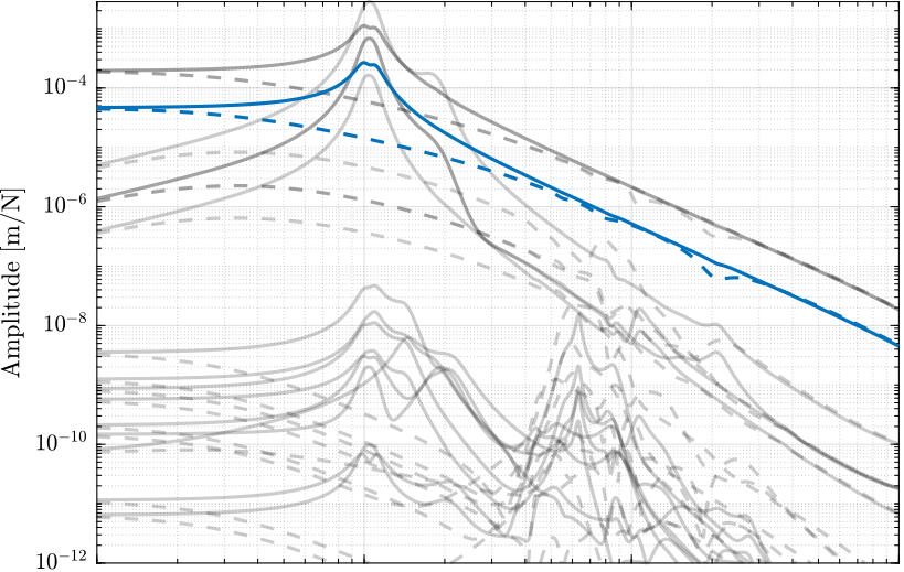
Figure 7: Coupling in the primary plant in the task with (dashed) and without (solid) Direct Velocity Feedback
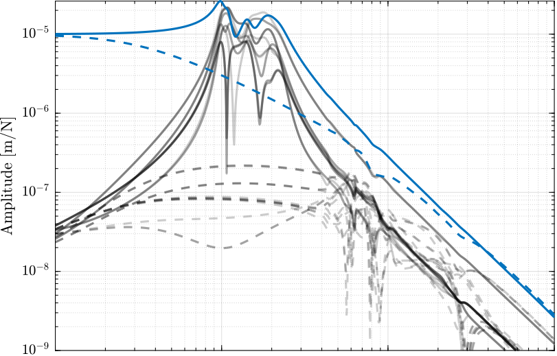
Figure 8: Coupling in the primary plant in the space of the legs with (dashed) and without (solid) Direct Velocity Feedback
1.5 Effect of the Low Authority Control on the Sensibility to Disturbances
We may now see how Decentralized Direct Velocity Feedback changes the sensibility to disturbances, namely:
- Ground motion
- Spindle and Translation stage vibrations
- Direct forces applied to the sample
To simplify the analysis, we here only consider the vertical direction, thus, we will look at the transfer functions:
- from vertical ground motion \(D_{w,z}\) to the vertical position error of the sample \(E_z\)
- from vertical vibration forces of the spindle \(F_{R_z,z}\) to \(E_z\)
- from vertical vibration forces of the translation stage \(F_{T_y,z}\) to \(E_z\)
- from vertical direct forces (such as cable forces) \(F_{d,z}\) to \(E_z\)
The norm of these transfer functions are shown in Figure 9.
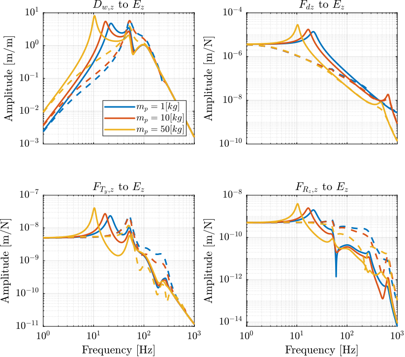
Figure 9: Norm of the transfer function from vertical disturbances to vertical position error with (dashed) and without (solid) Direct Velocity Feedback applied
Decentralized Direct Velocity Feedback is shown to increase the effect of stages vibrations at high frequency and to reduce the effect of ground motion and direct forces at low frequency.
1.6 Conclusion
2 Primary Control in the leg space
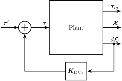
In this section we implement the control architecture shown in Figure 10 consisting of:
- an inner loop with a decentralized direct velocity feedback control
- an outer loop where the controller \(\bm{K}_\mathcal{L}\) is designed in the frame of the legs

Figure 10: Cascade Control Architecture. The inner loop consist of a decentralized Direct Velocity Feedback. The outer loop consist of position control in the leg’s space
The controller for decentralized direct velocity feedback is the one designed in Section 1.
2.1 Plant in the leg space
We now look at the transfer function matrix from \(\bm{\tau}^\prime\) to \(\bm{\epsilon}_{\mathcal{X}_n}\) for the design of \(\bm{K}_\mathcal{L}\).
The diagonal elements of the transfer function matrix from \(\bm{\tau}^\prime\) to \(\bm{\epsilon}_{\mathcal{X}_n}\) for the three considered masses are shown in Figure 11.
The plant dynamics below \(100\ [Hz]\) is only slightly dependent on the payload mass.
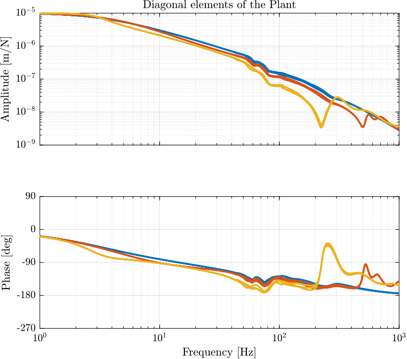
Figure 11: Diagonal elements of the transfer function matrix from \(\bm{\tau}^\prime\) to \(\bm{\epsilon}_{\mathcal{X}_n}\) for the three considered masses
2.2 Control in the leg space
We design a diagonal controller with all the same diagonal elements.
The requirements for the controller are:
- Crossover frequency of around 100Hz
- Stable for all the considered payload masses
- Sufficient phase and gain margin
- Integral action at low frequency
The design controller is as follows:
- Lead centered around the crossover
- An integrator below 10Hz
- A low pass filter at 250Hz
The loop gain is shown in Figure 12.
h = 2.0;
Kl = 2e7 * eye(6) * ...
     1/h*(s/(2*pi*100/h) + 1)/(s/(2*pi*100*h) + 1) * ...
     1/h*(s/(2*pi*200/h) + 1)/(s/(2*pi*200*h) + 1) * ...
     (s/2/pi/10 + 1)/(s/2/pi/10) * ...
     1/(1 + s/2/pi/300);
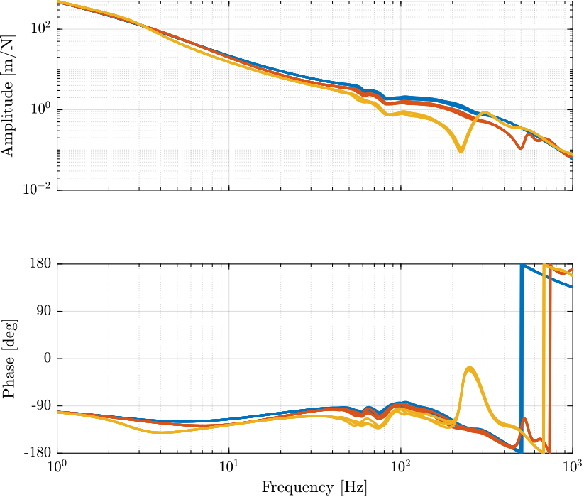
Figure 12: Loop gain for the primary plant
Finally, we include the Jacobian in the control and we ignore the measurement of the vertical rotation as for the real system.
load('mat/stages.mat', 'nano_hexapod');
K = Kl*nano_hexapod.J*diag([1, 1, 1, 1, 1, 0]);
2.3 Sensibility to Disturbances and Noise Budget
We identify the transfer function from disturbances to the position error of the sample when the HAC-LAC control is applied.
We compare the norm of these transfer function for the vertical direction when no control is applied and when HAC-LAC control is applied: Figure 13.
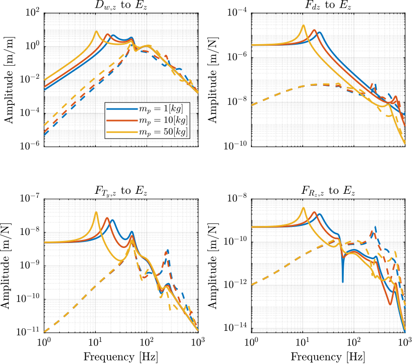
Figure 13: Sensibility to disturbances when the HAC-LAC control is applied
Then, we load the Power Spectral Density of the perturbations and we look at the obtained PSD of the displacement error in the vertical direction due to the disturbances:
- Figure 14: Amplitude Spectral Density of the vertical position error due to both the vertical ground motion and the vertical vibrations of the spindle
- Figure 15: Comparison of the Amplitude Spectral Density of the vertical position error in Open Loop and with the HAC-DVF Control
- Figure 16: Comparison of the Cumulative Amplitude Spectrum of the vertical position error in Open Loop and with the HAC-DVF Control
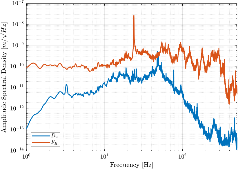
Figure 14: Amplitude Spectral Density of the vertical position error of the sample when the HAC-DVF control is applied due to both the ground motion and spindle vibrations
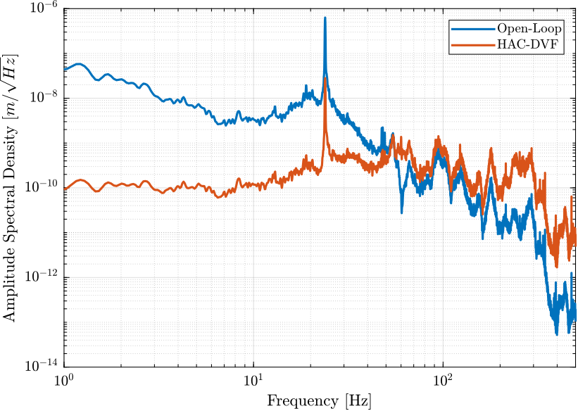
Figure 15: Amplitude Spectral Density of the vertical position error of the sample in Open-Loop and when the HAC-DVF control is applied
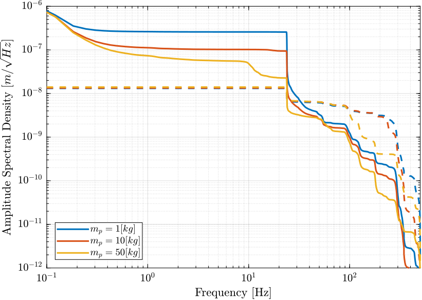
Figure 16: Cumulative Amplitude Spectrum of the vertical position error of the sample in Open-Loop and when the HAC-DVF control is applied
2.4 Simulations
Let’s now simulate a tomography experiment. To do so, we include all disturbances except vibrations of the translation stage.
initializeDisturbances();
initializeSimscapeConfiguration('gravity', false);
initializeLoggingConfiguration('log', 'all');
And we run the simulation for all three payload Masses.
2.5 Results
Let’s now see how this controller performs.
First, we compute the Power Spectral Density of the sample’s position error and we compare it with the open loop case in Figure 17.
Similarly, the Cumulative Amplitude Spectrum is shown in Figure 18.
Finally, the time domain position error signals are shown in Figure 19.
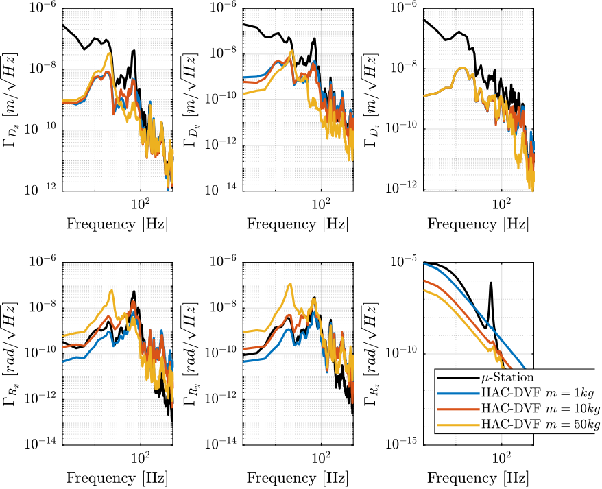
Figure 17: Amplitude Spectral Density of the position error in Open Loop and with the HAC-LAC controller
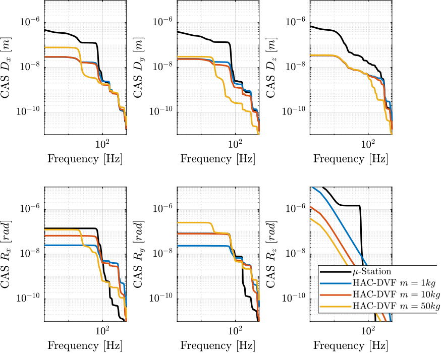
Figure 18: Cumulative Amplitude Spectrum of the position error in Open Loop and with the HAC-LAC controller
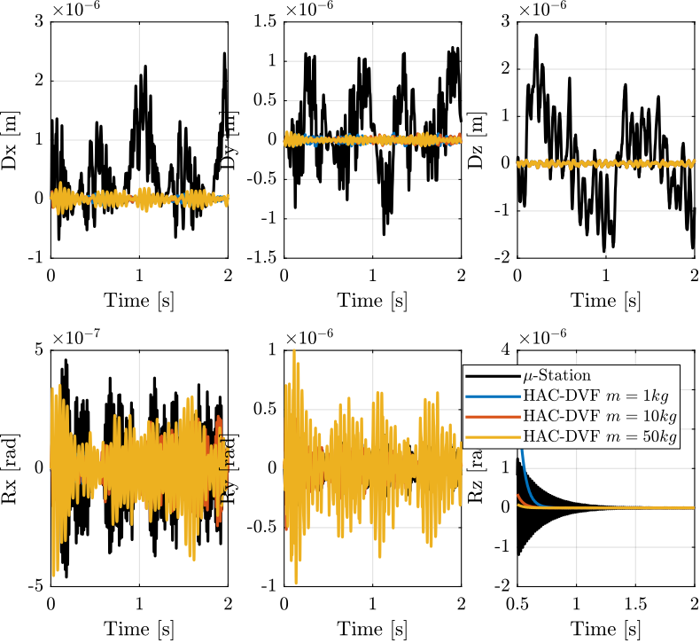
Figure 19: Position Error of the sample during a tomography experiment when no control is applied and with the HAC-DVF control architecture
2.6 Conclusion
3 Primary Control in the task space
In this section, the control architecture shown in Figure 20 is applied and consists of:
- an inner Low Authority Control loop consisting of a decentralized direct velocity control controller
- an outer loop with the primary controller \(\bm{K}_\mathcal{X}\) designed in the task space
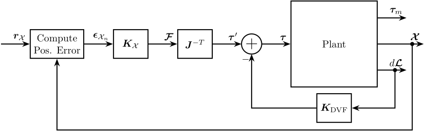
Figure 20: HAC-LAC architecture
3.1 Plant in the task space
Let’s look \(\bm{G}_\mathcal{X}(s)\).
3.2 Control in the task space
Kx = tf(zeros(6));

h = 2.5;
Kx(1,1) = 3e7 * ...
          1/h*(s/(2*pi*100/h) + 1)/(s/(2*pi*100*h) + 1) * ...
          (s/2/pi/1 + 1)/(s/2/pi/1);

Kx(2,2) = Kx(1,1);

h = 2.5;
Kx(3,3) = 3e7 * ...
          1/h*(s/(2*pi*100/h) + 1)/(s/(2*pi*100*h) + 1) * ...
          (s/2/pi/1 + 1)/(s/2/pi/1);
h = 1.5;
Kx(4,4) = 5e5 * ...
          1/h*(s/(2*pi*100/h) + 1)/(s/(2*pi*100*h) + 1) * ...
          (s/2/pi/1 + 1)/(s/2/pi/1);

Kx(5,5) = Kx(4,4);

h = 1.5;
Kx(6,6) = 5e4 * ...
          1/h*(s/(2*pi*30/h) + 1)/(s/(2*pi*30*h) + 1) * ...
          (s/2/pi/1 + 1)/(s/2/pi/1);
3.2.1 Stability
for i = 1:length(Ms)
    isstable(feedback(Gm_x{i}*Kx, eye(6), -1))
end
3.3 Simulation
3.4 Conclusion