Control of the NASS with Voice coil actuators

1. Initialization
2. Low Authority Control - Integral Force Feedback \(\bm{K}_\text{IFF}\)
3. High Authority Control in the joint space - \(\bm{K}_\mathcal{L}\)
4. On the usefulness of the High Authority Control loop / Linearization loop
5. Primary Controller in the task space - \(\bm{K}_\mathcal{X}\)
6. Simulation
7. Results

The goal here is to study the use of a voice coil based nano-hexapod. That is to say a nano-hexapod with a very small stiffness.

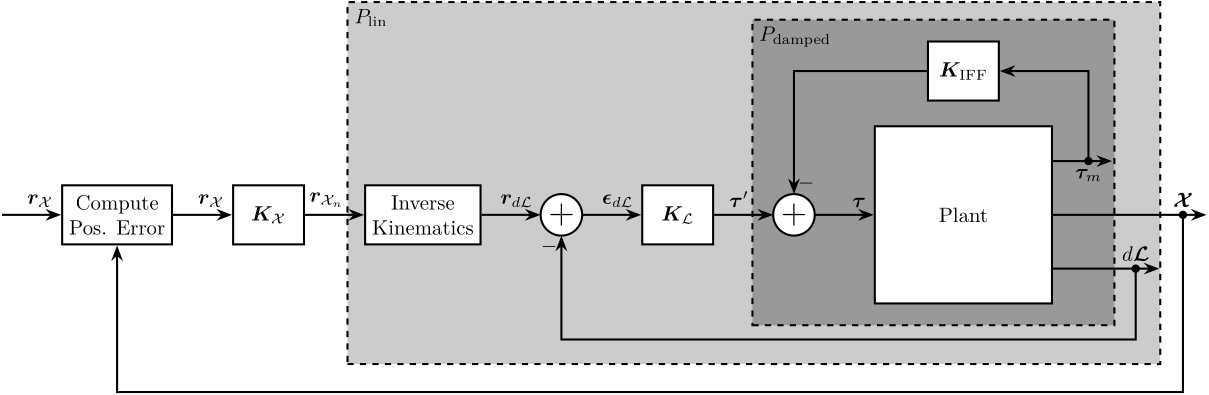
Figure 1: Cascaded Control consisting of (from inner to outer loop): IFF, Linearization Loop, Tracking Control in the frame of the Legs

1 Initialization

We initialize all the stages with the default parameters.

initializeGround();
initializeGranite();
initializeTy();
initializeRy();
initializeRz();
initializeMicroHexapod();
initializeAxisc();
initializeMirror();

The nano-hexapod is a voice coil based hexapod and the sample has a mass of 1kg.

initializeNanoHexapod('actuator', 'lorentz');
initializeSample('mass', 1);

We set the references that corresponds to a tomography experiment.

initializeReferences('Rz_type', 'rotating', 'Rz_period', 1);

initializeDisturbances();

initializeController('type', 'cascade-hac-lac');

initializeSimscapeConfiguration('gravity', true);

We log the signals.

initializeLoggingConfiguration('log', 'all');

Kx = tf(zeros(6));
Kl = tf(zeros(6));
Kiff = tf(zeros(6));

2 Low Authority Control - Integral Force Feedback \(\bm{K}_\text{IFF}\)

2.1 Identification

Let’s first identify the plant for the IFF controller.

%% Name of the Simulink File
mdl = 'nass_model';

%% Input/Output definition
clear io; io_i = 1;
io(io_i) = linio([mdl, '/Controller'],    1, 'openinput');               io_i = io_i + 1; % Actuator Inputs
io(io_i) = linio([mdl, '/Micro-Station'], 3, 'openoutput', [], 'Fnlm');  io_i = io_i + 1; % Force Sensors

%% Run the linearization
G_iff = linearize(mdl, io, 0);
G_iff.InputName  = {'Fnl1', 'Fnl2', 'Fnl3', 'Fnl4', 'Fnl5', 'Fnl6'};
G_iff.OutputName = {'Fnlm1', 'Fnlm2', 'Fnlm3', 'Fnlm4', 'Fnlm5', 'Fnlm6'};

2.2 Plant

The obtained plant for IFF is shown in Figure 2.

Figure 2: IFF Plant (png, pdf)

2.3 Root Locus

As seen in the root locus (Figure 3, no damping can be added to modes corresponding to the resonance of the micro-station.

However, critical damping can be achieve for the resonances of the nano-hexapod as shown in the zoomed part of the root (Figure 3, left part). The maximum damping is obtained for a control gain of \(\approx 70\).

Figure 3: Root Locus for the IFF control (png, pdf)

2.4 Controller and Loop Gain

We create the \(6 \times 6\) diagonal Integral Force Feedback controller. The obtained loop gain is shown in Figure 4.

Kiff = -70/s*eye(6);

Figure 4: Obtained Loop gain the IFF Control (png, pdf)

3 High Authority Control in the joint space - \(\bm{K}_\mathcal{L}\)

3.1 Identification of the damped plant

Let’s identify the dynamics from \(\bm{\tau}^\prime\) to \(d\bm{\mathcal{L}}\) as shown in Figure 1.

%% Name of the Simulink File
mdl = 'nass_model';

%% Input/Output definition
clear io; io_i = 1;
io(io_i) = linio([mdl, '/Controller'],    1, 'input');               io_i = io_i + 1; % Actuator Inputs
io(io_i) = linio([mdl, '/Micro-Station'], 3, 'output', [], 'Dnlm');  io_i = io_i + 1; % Leg Displacement

%% Run the linearization
Gl = linearize(mdl, io, 0);
Gl.InputName  = {'Fnl1', 'Fnl2', 'Fnl3', 'Fnl4', 'Fnl5', 'Fnl6'};
Gl.OutputName = {'Dnlm1', 'Dnlm2', 'Dnlm3', 'Dnlm4', 'Dnlm5', 'Dnlm6'};

There are some unstable poles in the Plant with very small imaginary parts. These unstable poles are probably not physical, and they disappear when taking the minimum realization of the plant.

isstable(Gl)
Gl = minreal(Gl);
isstable(Gl)

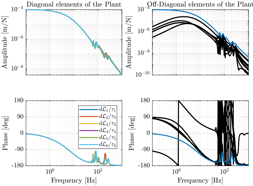
3.2 Obtained Plant

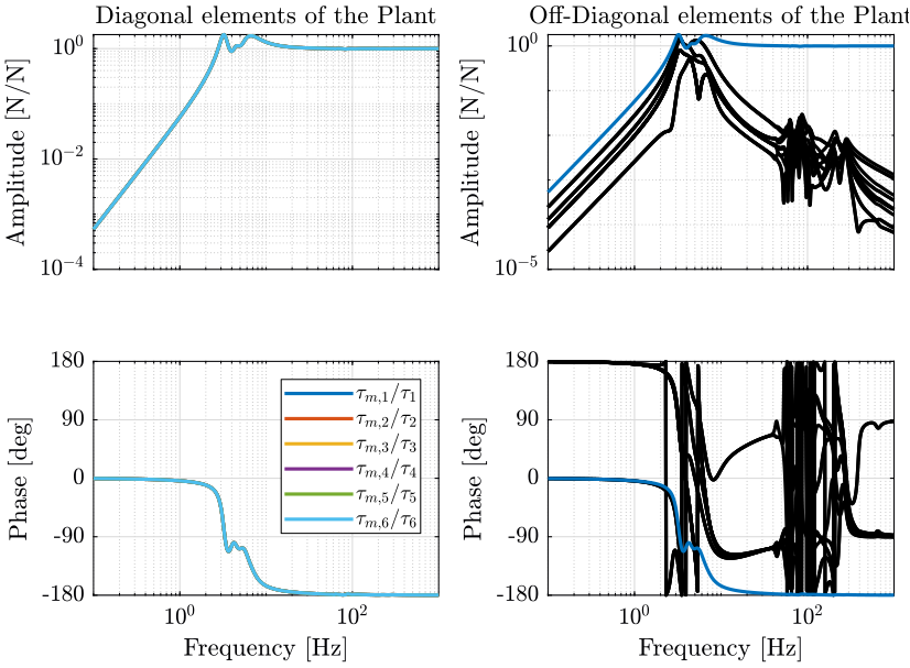
The obtained dynamics is shown in Figure 5.

Few things can be said on the dynamics:

the dynamics of the diagonal elements are almost all the same
the system is well decoupled below the resonances of the nano-hexapod (1Hz)
the dynamics of the diagonal elements are almost equivalent to a critically damped mass-spring-system with some spurious resonances above 50Hz corresponding to the resonances of the micro-station

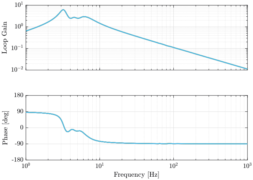
Figure 5: Plant for the High Authority Control in the Joint Space (png, pdf)

3.3 Controller Design and Loop Gain

As the plant is well decoupled, a diagonal plant is designed.

wc = 2*pi*5; % Bandwidth Bandwidth [rad/s]

h = 2; % Lead parameter

Kl = (1/h) * (1 + s/wc*h)/(1 + s/wc/h) * ... % Lead
     (1/h) * (1 + s/wc*h)/(1 + s/wc/h) * ... % Lead
     (s + 2*pi*10)/s * ... % Weak Integrator
     (s + 2*pi*1)/s * ... % Weak Integrator
     1/(1 + s/2/pi/10); % Low pass filter after crossover

% Normalization of the gain of have a loop gain of 1 at frequency wc
Kl = Kl.*diag(1./diag(abs(freqresp(Gl*Kl, wc))));

4 On the usefulness of the High Authority Control loop / Linearization loop

Let’s see what happens is we omit the HAC loop and we directly try to control the damped plant using the measurement of the sample with respect to the granite \(\bm{\mathcal{X}}\).

We can do that in two different ways:

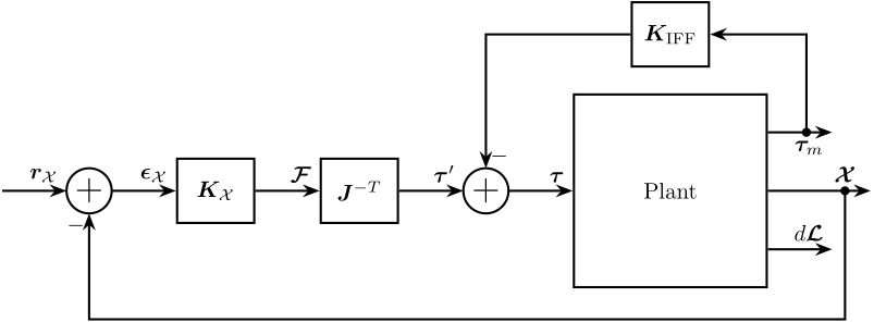
in the task space as shown in Figure 6
in the space of the legs as shown in Figure 7

Figure 6: IFF control + primary controller in the task space

Figure 7: HAC-LAC control architecture in the frame of the legs

4.1 Identification

initializeController('type', 'hac-iff');

%% Name of the Simulink File
mdl = 'nass_model';

%% Input/Output definition
clear io; io_i = 1;
io(io_i) = linio([mdl, '/Controller/HAC-IFF/Kx'],  1, 'input');    io_i = io_i + 1;
io(io_i) = linio([mdl, '/Tracking Error'], 1, 'output', [], 'En'); io_i = io_i + 1; % Position Errror

%% Run the linearization
G = linearize(mdl, io, 0);
G.InputName  = {'F1', 'F2', 'F3', 'F4', 'F5', 'F6'};
G.OutputName = {'Ex', 'Ey', 'Ez', 'Erx', 'Ery', 'Erz'};

isstable(G)
G = -minreal(G);
isstable(G)

4.2 Plant in the Task space

The obtained plant is shown in Figure

Gx = G*inv(nano_hexapod.J');

4.3 Plant in the Leg’s space

Gl = nano_hexapod.J*G;

5 Primary Controller in the task space - \(\bm{K}_\mathcal{X}\)

5.1 Identification of the linearized plant

We know identify the dynamics between \(\bm{r}_{\mathcal{X}_n}\) and \(\bm{r}_\mathcal{X}\).

%% Name of the Simulink File
mdl = 'nass_model';

%% Input/Output definition
clear io; io_i = 1;
io(io_i) = linio([mdl, '/Controller/Cascade-HAC-LAC/Kx'],  1, 'input'); io_i = io_i + 1;
io(io_i) = linio([mdl, '/Tracking Error'], 1, 'output', [], 'En');      io_i = io_i + 1; % Position Errror

%% Run the linearization
Gx = linearize(mdl, io, 0);
Gx.InputName  = {'rL1', 'rL2', 'rL3', 'rL4', 'rL5', 'rL6'};
Gx.OutputName = {'Ex', 'Ey', 'Ez', 'Erx', 'Ery', 'Erz'};

As before, we take the minimum realization.

isstable(Gx)
Gx = -minreal(Gx);
isstable(Gx)

5.2 Obtained Plant

5.3 Controller Design

wc = 2*pi*200; % Bandwidth Bandwidth [rad/s]

h = 2; % Lead parameter

Kx = (1/h) * (1 + s/wc*h)/(1 + s/wc/h) * ...
     (s + 2*pi*10)/s * ...
     (s + 2*pi*100)/s * ...
     1/(1+s/2/pi/500); % For Piezo
% Kx = (1/h) * (1 + s/wc*h)/(1 + s/wc/h) * (s + 2*pi*10)/s * (s + 2*pi*1)/s ; % For voice coil

% Normalization of the gain of have a loop gain of 1 at frequency wc
Kx = Kx.*diag(1./diag(abs(freqresp(Gx*Kx, wc))));

6 Simulation

load('mat/conf_simulink.mat');
set_param(conf_simulink, 'StopTime', '2');

And we simulate the system.

sim('nass_model');

cascade_hac_lac_lorentz = simout;
save('./mat/cascade_hac_lac.mat', 'cascade_hac_lac_lorentz', '-append');

7 Results

7.1 Load the simulation results

load('./mat/experiment_tomography.mat', 'tomo_align_dist');
load('./mat/cascade_hac_lac.mat', 'cascade_hac_lac', 'cascade_hac_lac_lorentz');

7.2 Control effort

7.3 Load the simulation results

n_av = 4;
han_win = hanning(ceil(length(cascade_hac_lac.Em.En.Data(:,1))/n_av));

t = cascade_hac_lac.Em.En.Time;
Ts = t(2)-t(1);

[pxx_ol, f] = pwelch(tomo_align_dist.Em.En.Data, han_win, [], [], 1/Ts);
[pxx_ca, ~] = pwelch(cascade_hac_lac.Em.En.Data, han_win, [], [], 1/Ts);
[pxx_vc, ~] = pwelch(cascade_hac_lac_lorentz.Em.En.Data, han_win, [], [], 1/Ts);