Amplified Piezoelectric Stack Actuator
Table of Contents
The presented model is based on souleille18_concep_activ_mount_space_applic.
The model represents the amplified piezo APA100M from Cedrat-Technologies (Figure 1). The parameters are shown in the table below.
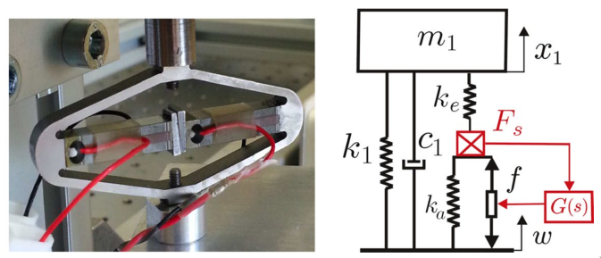
Figure 1: Picture of an APA100M from Cedrat Technologies. Simplified model of a one DoF payload mounted on such isolator
| Value | Meaning | |
|---|---|---|
| \(m\) | \(1\,[kg]\) | Payload mass |
| \(k_e\) | \(4.8\,[N/\mu m]\) | Stiffness used to adjust the pole of the isolator |
| \(k_1\) | \(0.96\,[N/\mu m]\) | Stiffness of the metallic suspension when the stack is removed |
| \(k_a\) | \(65\,[N/\mu m]\) | Stiffness of the actuator |
| \(c_1\) | \(10\,[N/(m/s)]\) | Added viscous damping |
1 Simplified Model
1.1 Parameters
m = 1; % [kg]

ke = 4.8e6; % [N/m]
ce = 5; % [N/(m/s)]
me = 0.001; % [kg]

k1 = 0.96e6; % [N/m]
c1 = 10; % [N/(m/s)]

ka = 65e6; % [N/m]
ca = 5; % [N/(m/s)]
ma = 0.001; % [kg]

h = 0.2; % [m]
IFF Controller:
Kiff = -8000/s;
1.2 Identification
Identification in open-loop.
%% Name of the Simulink File
mdl = 'amplified_piezo_model';

%% Input/Output definition
clear io; io_i = 1;
io(io_i) = linio([mdl, '/w'],  1, 'openinput');  io_i = io_i + 1; % Base Motion
io(io_i) = linio([mdl, '/f'],  1, 'openinput');  io_i = io_i + 1; % Actuator Inputs
io(io_i) = linio([mdl, '/F'],  1, 'openinput');  io_i = io_i + 1; % External Force

io(io_i) = linio([mdl, '/Fs'], 3, 'openoutput'); io_i = io_i + 1; % Force Sensors
io(io_i) = linio([mdl, '/x1'], 1, 'openoutput'); io_i = io_i + 1; % Mass displacement

G = linearize(mdl, io, 0);
G.InputName  = {'w', 'f', 'F'};
G.OutputName = {'Fs', 'x1'};
Identification in closed-loop.
%% Name of the Simulink File
mdl = 'amplified_piezo_model';

%% Input/Output definition
clear io; io_i = 1;
io(io_i) = linio([mdl, '/w'],  1, 'input');  io_i = io_i + 1; % Base Motion
io(io_i) = linio([mdl, '/f'],  1, 'input');  io_i = io_i + 1; % Actuator Inputs
io(io_i) = linio([mdl, '/F'],  1, 'input');  io_i = io_i + 1; % External Force

io(io_i) = linio([mdl, '/Fs'], 3, 'output'); io_i = io_i + 1; % Force Sensors
io(io_i) = linio([mdl, '/x1'], 1, 'output'); io_i = io_i + 1; % Mass displacement

Giff = linearize(mdl, io, 0);
Giff.InputName  = {'w', 'f', 'F'};
Giff.OutputName = {'Fs', 'x1'};
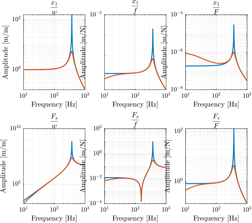
Figure 2: Matrix of transfer functions from input to output in open loop (blue) and closed loop (red)
1.3 Root Locus
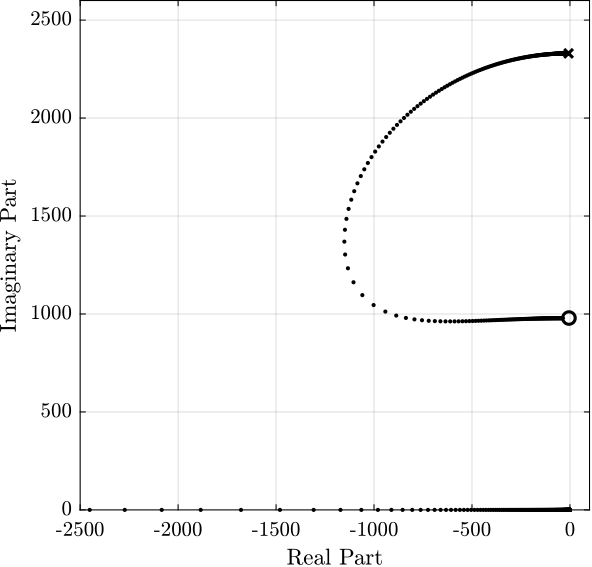
Figure 3: Root Locus
1.4 Analytical Model
If we apply the Newton’s second law of motion on the top mass, we obtain: \[ ms^2 x_1 = F + k_1 (w - x_1) + k_e (x_e - x_1) \]
Then, we can write that the measured force \(F_s\) is equal to: \[ F_s = k_a(w - x_e) + f = -k_e (x_1 - x_e) \] which gives: \[ x_e = \frac{k_a}{k_e + k_a} w + \frac{1}{k_e + k_a} f + \frac{k_e}{k_e + k_a} x_1 \]
Re-injecting that into the previous equations gives: \[ x_1 = F \frac{1}{ms^2 + k_1 + \frac{k_e k_a}{k_e + k_a}} + w \frac{k_1 + \frac{k_e k_a}{k_e + k_a}}{ms^2 + k_1 + \frac{k_e k_a}{k_e + k_a}} + f \frac{\frac{k_e}{k_e + k_a}}{ms^2 + k_1 + \frac{k_e k_a}{k_e + k_a}} \] \[ F_s = - F \frac{\frac{k_e k_a}{k_e + k_a}}{ms^2 + k_1 + \frac{k_e k_a}{k_e + k_a}} + w \frac{k_e k_a}{k_e + k_a} \Big( \frac{ms^2}{ms^2 + k_1 + \frac{k_e k_a}{k_e + k_a}} \Big) - f \frac{k_e}{k_e + k_a} \Big( \frac{ms^2 + k_1}{ms^2 + k_1 + \frac{k_e k_a}{k_e + k_a}} \Big) \]
Ga = 1/(m*s^2 + k1 + ke*ka/(ke + ka)) * ...
     [ 1 ,              k1 + ke*ka/(ke + ka)  , ke/(ke + ka) ;
      -ke*ka/(ke + ka), ke*ka/(ke + ka)*m*s^2 , -ke/(ke+ka)*(m*s^2 + k1)];
Ga.InputName = {'F', 'w', 'f'};
Ga.OutputName = {'x1', 'Fs'};
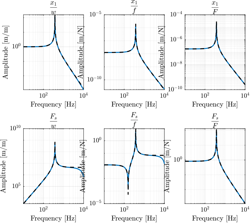
Figure 4: Comparison of the Identified Simscape Dynamics (solid) and the Analytical Model (dashed)
1.5 Analytical Analysis
For Integral Force Feedback Control, the plant is: \[ \frac{F_s}{f} = \frac{k_e}{k_e + k_a} \Big( \frac{ms^2 + k_1}{ms^2 + k_1 + \frac{k_e k_a}{k_e + k_a}} \Big) \]
As high frequency, this converge to: \[ \frac{F_s}{f} \underset{\omega\to\infty}{\longrightarrow} \frac{k_e}{k_e + k_a} \] And at low frequency: \[ \frac{F_s}{f} \underset{\omega\to 0}{\longrightarrow} \frac{k_e}{k_e + k_a} \frac{k_1}{k_1 + \frac{k_e k_a}{k_e + k_a}} \]
It has two complex conjugate zeros at: \[ z = \pm j \sqrt{\frac{k_1}{m}} \] And two complex conjugate poles at: \[ p = \pm j \sqrt{\frac{k_1 + \frac{k_e k_a}{k_e + k_a}}{m}} \]
If maximal damping is to be attained with IFF, the distance between the zero and the pole is to be maximized. Thus, we wish to maximize \(p/z\), which is equivalent as to minimize \(k_1\) and have \(k_e \approx k_a\) (supposing \(k_e + k_a \approx \text{cst}\)).
2 Rotating X-Y platform
2.1 Parameters
m = 1; % [kg]

ke = 4.8e6; % [N/m]
ce = 5; % [N/(m/s)]
me = 0.001; % [kg]

k1 = 0.96e6; % [N/m]
c1 = 10; % [N/(m/s)]

ka = 65e6; % [N/m]
ca = 5; % [N/(m/s)]
ma = 0.001; % [kg]

h = 0.2; % [m]
Kiff = tf(0);
2.2 Identification
Rotating speed in rad/s:
Ws = 2*pi*[0, 1, 10, 100];
Gs = {zeros(length(Ws), 1)};
Identification in open-loop.
%% Name of the Simulink File
mdl = 'amplified_piezo_xy_rotating_stage';

%% Input/Output definition
clear io; io_i = 1;
io(io_i) = linio([mdl, '/fx'],  1, 'openinput');  io_i = io_i + 1;
io(io_i) = linio([mdl, '/fy'],  1, 'openinput');  io_i = io_i + 1;

io(io_i) = linio([mdl, '/Fs'], 1, 'openoutput'); io_i = io_i + 1;
io(io_i) = linio([mdl, '/Fs'], 2, 'openoutput'); io_i = io_i + 1;

for i = 1:length(Ws)
    ws = Ws(i);
    G = linearize(mdl, io, 0);
    G.InputName  = {'fx', 'fy'};
    G.OutputName = {'Fsx', 'Fsy'};
    Gs(i) = {G};
end
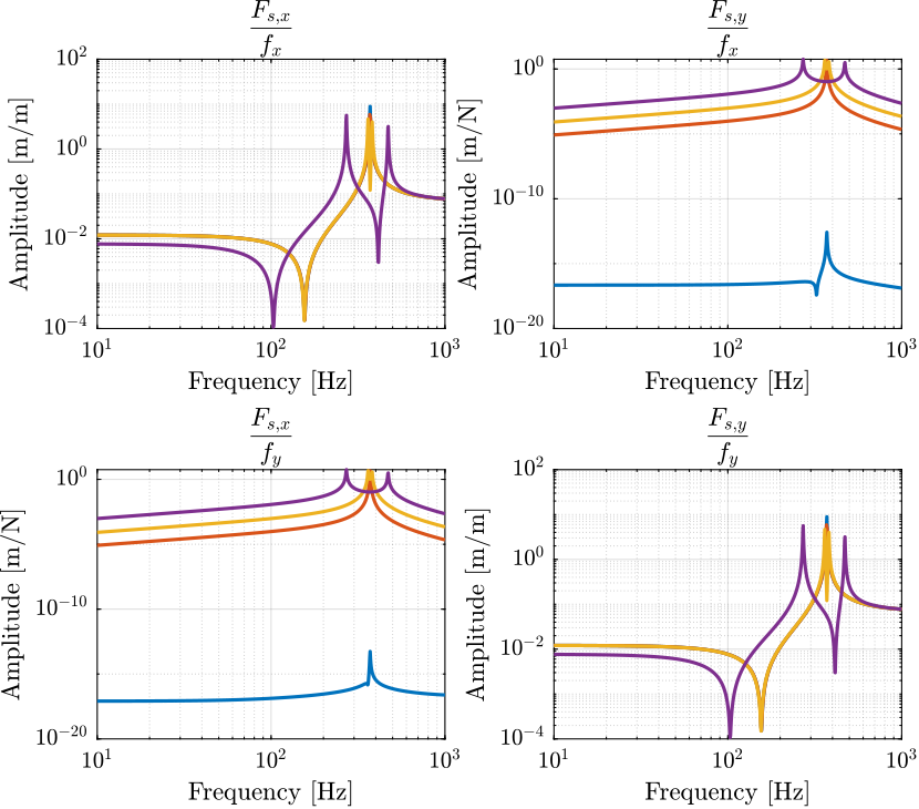
Figure 5: Transfer function matrix from forces to force sensors for multiple rotation speed
2.3 Root Locus
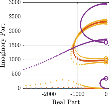
Figure 6: Root locus for 3 rotating speed
2.4 Analysis
The negative stiffness induced by the rotation is equal to \(m \omega_0^2\). Thus, the maximum rotation speed where IFF can be applied is: \[ \omega_\text{max} = \sqrt{\frac{k_1}{m}} \approx 156\,[Hz] \]
Let’s verify that.
Ws = 2*pi*[140, 160];
Identification
%% Name of the Simulink File
mdl = 'amplified_piezo_xy_rotating_stage';

%% Input/Output definition
clear io; io_i = 1;
io(io_i) = linio([mdl, '/fx'],  1, 'openinput');  io_i = io_i + 1;
io(io_i) = linio([mdl, '/fy'],  1, 'openinput');  io_i = io_i + 1;

io(io_i) = linio([mdl, '/Fs'], 1, 'openoutput'); io_i = io_i + 1;
io(io_i) = linio([mdl, '/Fs'], 2, 'openoutput'); io_i = io_i + 1;

for i = 1:length(Ws)
    ws = Ws(i);
    G = linearize(mdl, io, 0);
    G.InputName  = {'fx', 'fy'};
    G.OutputName = {'Fsx', 'Fsy'};
    Gs(i) = {G};
end
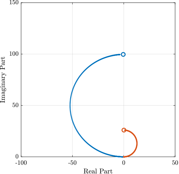
Figure 7: Root Locus for the two considered rotation speed. For the red curve, the system is unstable.
3 Stewart Platform with Amplified Actuators
3.1 Initialization
initializeGround();
initializeGranite();
initializeTy();
initializeRy();
initializeRz();
initializeMicroHexapod();
initializeAxisc();
initializeMirror();

initializeSimscapeConfiguration();
initializeDisturbances('enable', false);
initializeLoggingConfiguration('log', 'none');

initializeController('type', 'hac-iff');
We set the stiffness of the payload fixation:
Kp = 1e8; % [N/m]
3.2 Identification
K = tf(zeros(6));
Kiff = tf(zeros(6));
We identify the system for the following payload masses:
Ms = [1, 10, 50];
The nano-hexapod has the following leg’s stiffness and damping.
initializeNanoHexapod('actuator', 'amplified');
3.3 Controller Design
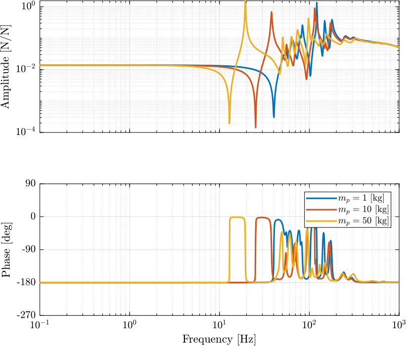
Figure 8: Dynamics for the Integral Force Feedback for three payload masses
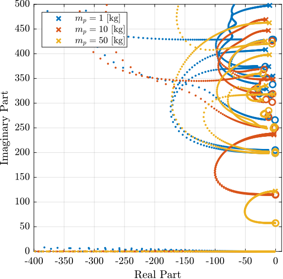
Figure 9: Root Locus for the IFF control for three payload masses
Damping as function of the gain
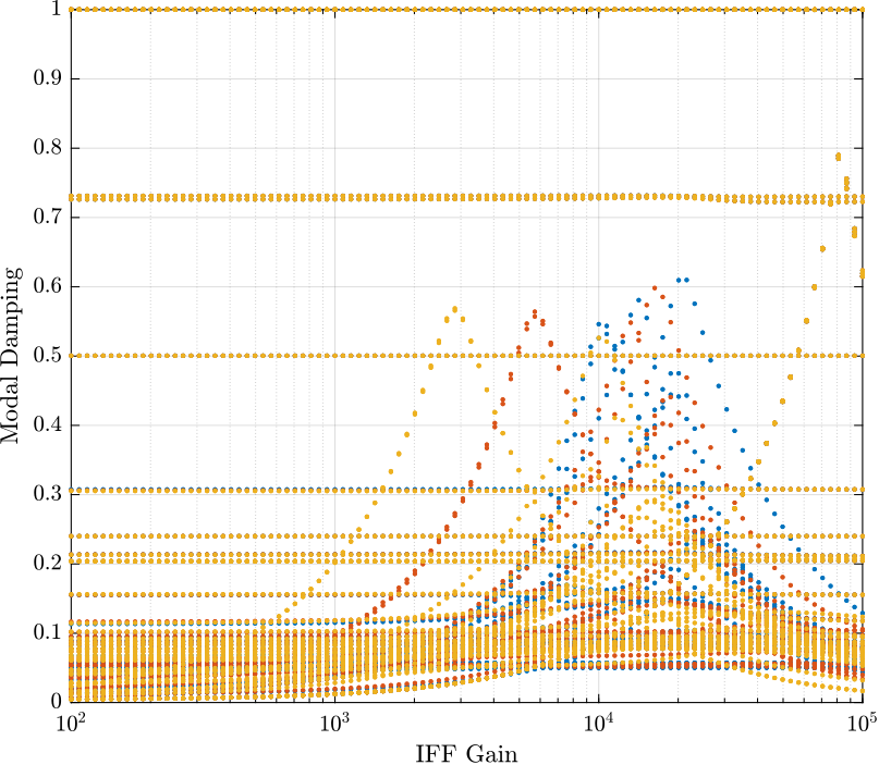
Figure 10: Damping ratio of the poles as a function of the IFF gain
Finally, we use the following controller for the Decentralized Direct Velocity Feedback:
Kiff = -1e4/s*eye(6);
3.4 Effect of the Low Authority Control on the Primary Plant
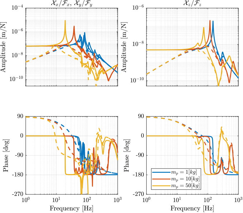
Figure 11: Primary plant in the task space with (dashed) and without (solid) IFF
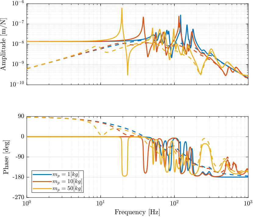
Figure 12: Primary plant in the space of the legs with (dashed) and without (solid) IFF
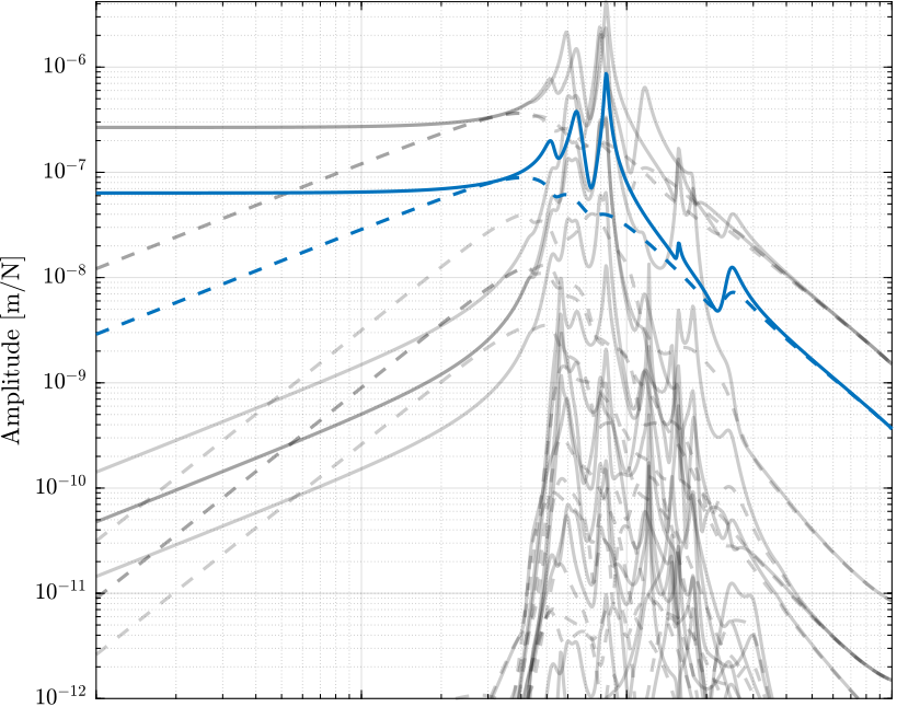
Figure 13: Coupling in the primary plant in the task with (dashed) and without (solid) IFF
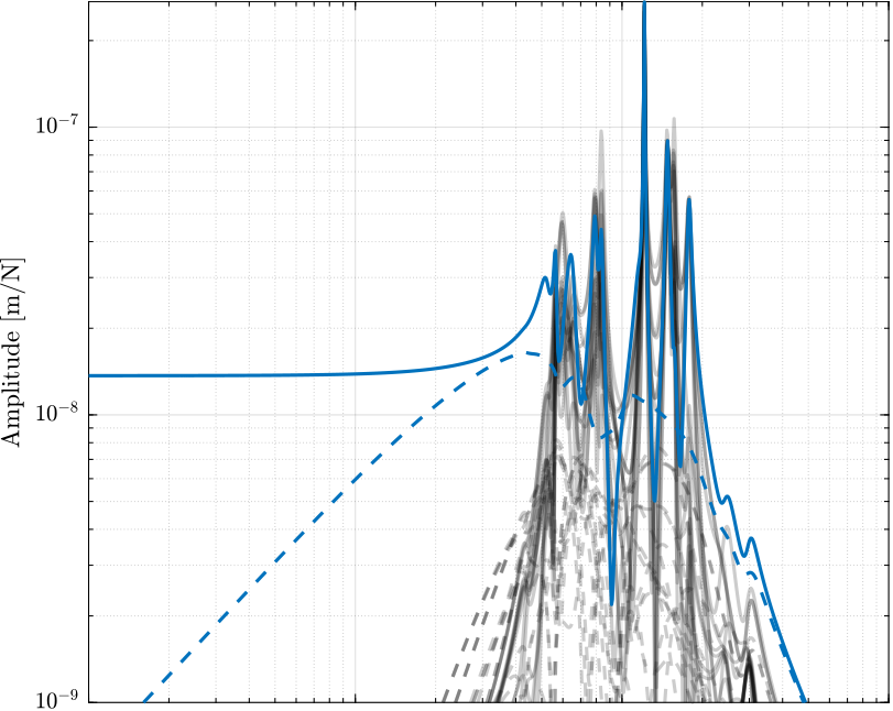
Figure 14: Coupling in the primary plant in the space of the legs with (dashed) and without (solid) IFF
3.5 Effect of the Low Authority Control on the Sensibility to Disturbances
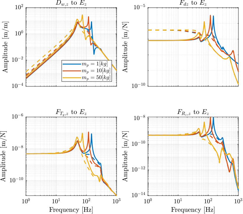
Figure 15: Norm of the transfer function from vertical disturbances to vertical position error with (dashed) and without (solid) Integral Force Feedback applied