Cascade Control applied on the Simscape Model
Table of Contents
The control architecture we wish here to study is shown in Figure 1.
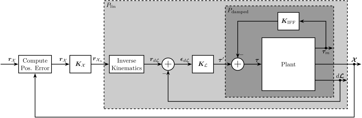
Figure 1: Cascaded Control consisting of (from inner to outer loop): IFF, Linearization Loop, Tracking Control in the frame of the Legs
This cascade control is designed in three steps:
- In section 2: an active damping controller is designed. This is based on the Integral Force Feedback and applied in a decentralized way
- In section 3: a decentralized tracking control is designed in the frame of the legs. This controller is based on the displacement of each of the legs
- In section 4: a controller is designed in the task space in order to follow the wanted reference path corresponding to the sample position with respect to the granite
1 Initialization
We initialize all the stages with the default parameters.
initializeGround();
initializeGranite();
initializeTy();
initializeRy();
initializeRz();
initializeMicroHexapod();
initializeAxisc();
initializeMirror();
The nano-hexapod is a piezoelectric hexapod and the sample has a mass of 50kg.
initializeNanoHexapod('actuator', 'piezo');
initializeSample('mass', 1);
We set the references that corresponds to a tomography experiment.
initializeReferences('Rz_type', 'rotating', 'Rz_period', 1);
initializeDisturbances();
Open Loop.
initializeController('type', 'cascade-hac-lac');
And we put some gravity.
initializeSimscapeConfiguration('gravity', true);
We log the signals.
initializeLoggingConfiguration('log', 'all');
Kx = tf(zeros(6));
Kl = tf(zeros(6));
Kiff = tf(zeros(6));
2 Low Authority Control - Integral Force Feedback \(\bm{K}_\text{IFF}\)
2.1 Identification
Let’s first identify the plant for the IFF controller.
%% Name of the Simulink File
mdl = 'nass_model';

%% Input/Output definition
clear io; io_i = 1;
io(io_i) = linio([mdl, '/Controller'],    1, 'openinput');               io_i = io_i + 1; % Actuator Inputs
io(io_i) = linio([mdl, '/Micro-Station'], 3, 'openoutput', [], 'Fnlm');  io_i = io_i + 1; % Force Sensors

%% Run the linearization
G_iff = linearize(mdl, io, 0);
G_iff.InputName  = {'Fnl1', 'Fnl2', 'Fnl3', 'Fnl4', 'Fnl5', 'Fnl6'};
G_iff.OutputName = {'Fnlm1', 'Fnlm2', 'Fnlm3', 'Fnlm4', 'Fnlm5', 'Fnlm6'};
2.3 Root Locus

3 High Authority Control in the joint space - \(\bm{K}_\mathcal{L}\)
3.1 Identification of the damped plant
We now identify the transfer function from \(\tau^\prime\) to \(d\bm{\mathcal{L}}\) as shown in Figure 1.
%% Name of the Simulink File
mdl = 'nass_model';

%% Input/Output definition
clear io; io_i = 1;
io(io_i) = linio([mdl, '/Controller'],    1, 'input');               io_i = io_i + 1; % Actuator Inputs
io(io_i) = linio([mdl, '/Micro-Station'], 3, 'output', [], 'Dnlm');  io_i = io_i + 1; % Leg Displacement

%% Run the linearization
Gl = linearize(mdl, io, 0);
Gl.InputName  = {'Fnl1', 'Fnl2', 'Fnl3', 'Fnl4', 'Fnl5', 'Fnl6'};
Gl.OutputName = {'Dnlm1', 'Dnlm2', 'Dnlm3', 'Dnlm4', 'Dnlm5', 'Dnlm6'};
There are some unstable poles in the Plant with very small imaginary parts. These unstable poles are probably not physical, and they disappear when taking the minimum realization of the plant.
isstable(Gl)
Gl = minreal(Gl);
isstable(Gl)
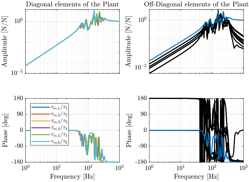
3.2 Obtained Plant

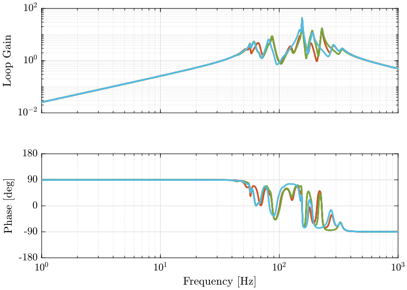
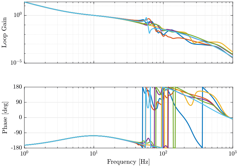
3.3 Controller Design and Loop Gain
The controller consists of:
- A pure integrator
- A Second integrator up to half the wanted bandwidth
- A Lead around the cross-over frequency
- A low pass filter with a cut-off equal to two times the wanted bandwidth
wc = 2*pi*400; % Bandwidth Bandwidth [rad/s]

h = 2; % Lead parameter

% Kl = (1/h) * (1 + s/wc*h)/(1 + s/wc/h) * wc/s * ((s/wc*2 + 1)/(s/wc*2)) * (1/(1 + s/wc/2));
Kl = (1/h) * (1 + s/wc*h)/(1 + s/wc/h) * (1/h) * (1 + s/wc*h)/(1 + s/wc/h) * wc/s;

% Normalization of the gain of have a loop gain of 1 at frequency wc
Kl = Kl.*diag(1./diag(abs(freqresp(Gl*Kl, wc))));
4 Primary Controller in the task space - \(\bm{K}_\mathcal{X}\)
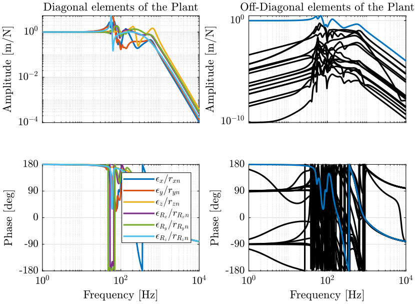
4.1 Identification of the linearized plant
We know identify the dynamics between \(\bm{r}_{\mathcal{X}_n}\) and \(\bm{r}_\mathcal{X}\).
%% Name of the Simulink File
mdl = 'nass_model';

%% Input/Output definition
clear io; io_i = 1;
io(io_i) = linio([mdl, '/Controller/Cascade-HAC-LAC/Kx'],  1, 'input'); io_i = io_i + 1;
io(io_i) = linio([mdl, '/Tracking Error'], 1, 'output', [], 'En');      io_i = io_i + 1; % Position Errror

%% Run the linearization
Gx = linearize(mdl, io, 0);
Gx.InputName  = {'rL1', 'rL2', 'rL3', 'rL4', 'rL5', 'rL6'};
Gx.OutputName = {'Ex', 'Ey', 'Ez', 'Erx', 'Ery', 'Erz'};
As before, we take the minimum realization.
isstable(Gx)
Gx = minreal(Gx);
isstable(Gx)
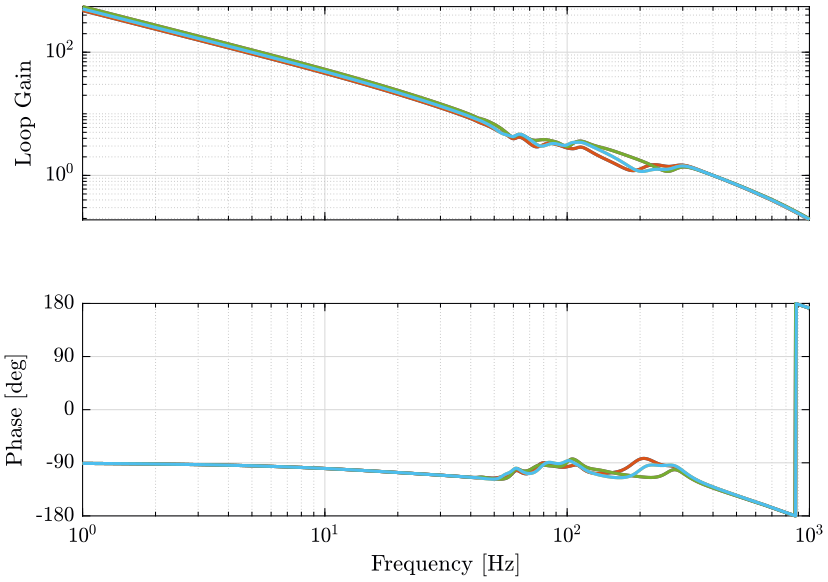
4.3 Controller Design
wc = 2*pi*10; % Bandwidth Bandwidth [rad/s]

h = 2; % Lead parameter

Kx = (1/h) * (1 + s/wc*h)/(1 + s/wc/h) * wc/s * (s + 2*pi*5)/s * 1/(1+s/2/pi/20);

% Normalization of the gain of have a loop gain of 1 at frequency wc
Kx = Kx.*diag(1./diag(abs(freqresp(Gx*Kx, wc))));
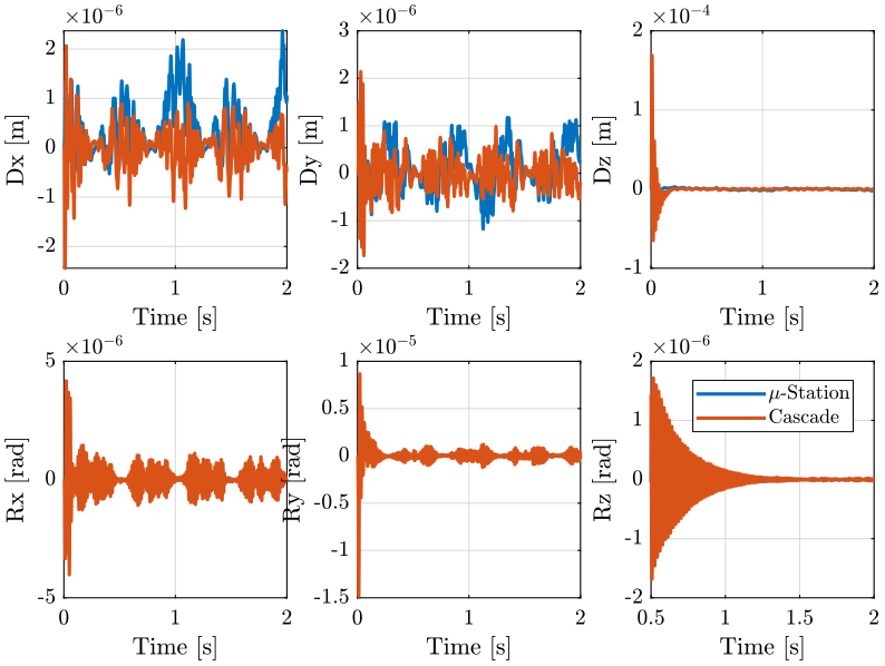
5 Simulation
load('mat/conf_simulink.mat');
set_param(conf_simulink, 'StopTime', '2');
And we simulate the system.
sim('nass_model');
cascade_hac_lac = simout;
save('./mat/cascade_hac_lac.mat', 'cascade_hac_lac');
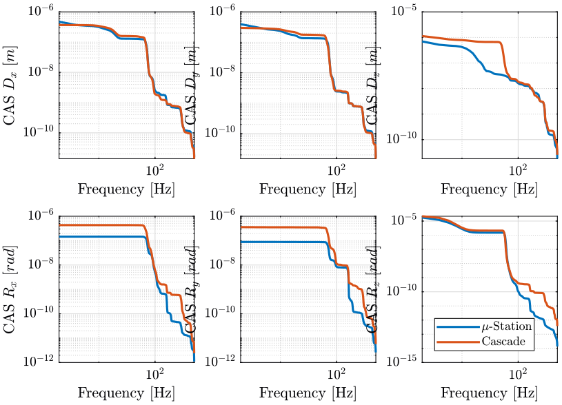
6 Results
load('./mat/experiment_tomography.mat', 'tomo_align_dist');
load('./mat/cascade_hac_lac.mat', 'cascade_hac_lac');
n_av = 4;
han_win = hanning(ceil(length(cascade_hac_lac.Em.En.Data(:,1))/n_av));
t = cascade_hac_lac.Em.En.Time;
Ts = t(2)-t(1);

[pxx_ol, f] = pwelch(tomo_align_dist.Em.En.Data, han_win, [], [], 1/Ts);
[pxx_ca, ~] = pwelch(cascade_hac_lac.Em.En.Data, han_win, [], [], 1/Ts);
