Control of the Nano-Active-Stabilization-System
Table of Contents
- 1. Control Configuration - Introduction
- 2. Tracking Control in the Frame of the Nano-Hexapod - Basic Architectures
- 3. Active Damping Architecture - Collocated Control (link)
- 4. HAC-LAC Architectures (link)
- 4.1. HAC-LAC using IFF and Tracking control in the frame of the Legs
- 4.2. HAC-LAC using IFF and Tracking control in the Cartesian frame
- 4.3. HAC-LAC using IFF - the HAC controller is positioning the sample w.r.t. the granite in the task space
- 4.4. HAC-LAC using IFF - the HAC controller is positioning the sample w.r.t. the granite in the space of the legs
- 4.5. HAC-LAC using DVF - the HAC controller is positioning the sample w.r.t. the granite in the task space
- 4.6. HAC-LAC using DVF - the HAC controller is positioning the sample w.r.t. the granite in the space of the legs
- 5. Cascade Architectures (link)
- 6. Force Control (link)
- 7. Other Control Architectures
The system consist of the following inputs and outputs (Figure 1):
- \(\bm{\tau}\): Forces applied in each leg
- \(\bm{\tau}_m\): Force sensor located in each leg
- \(\bm{\mathcal{X}}\): Measurement of the payload position with respect to the granite
- \(d\bm{\mathcal{L}}\): Measurement of the (small) relative motion of each leg
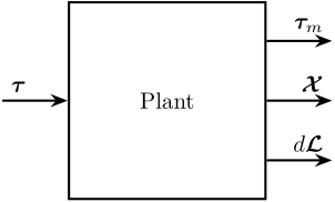
Figure 1: Block diagram with the inputs and outputs of the system
In order to position the Sample with respect to the granite, we must use the measurement \(\bm{\mathcal{X}}\) in the control loop. The wanted position of the sample with respect to the granite is represented by \(\bm{r}_\mathcal{X}\). From \(\bm{r}_\mathcal{X}\) and \(\bm{\mathcal{X}}\), we can compute the required small change of pose of the nano-hexapod’s top platform expressed in the frame of the nano-hexapod’s base as shown in Figure 2.
This can we considered as:
- the position error \(\bm{\epsilon}_{\mathcal{X}_n}\) expressed in a frame attach to the base of the nano-hexapod
- the wanted (small) pose displacement \(\bm{r}_{d\mathcal{X}_n}\) of the nano-hexapod mobile platform with respect to its base
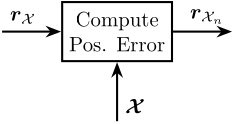
Figure 2: Block diagram corresponding to the computation of the position error in the frame of the nano-hexapod
In this document, we see how the different outputs of the system can be used to control of position \(\bm{\mathcal{X}}\).
1 Control Configuration - Introduction
In this section, we discuss the control configuration for the NASS.
From (Skogestad and Postlethwaite 2007):
We define the control configuration to be the restrictions imposed on the overall controller \(K\) by decomposing it into a set of local controllers with predetermined links and with a possibly predetermined design sequence where subcontrollers are designed locally.
Some elements used to build up a specific control configuration are:
- Cascade controllers. The output from one controller is the input to another
- Decentralized controllers. The control system consists of independent feedback controllers which interconnect a subset of the output measurements with a subset of the manipulated inputs. These subsets should not be used by any other controller
- Feedforward elements. Link measured disturbances and manipulated inputs
- Decoupling elements. Link one set of manipulated inputs with another set of manipulated inputs. They are used to improve the performance of decentralized control systems.
Decoupling elements will be used to convert quantities from the joint space to the task space and vice-versa.
Decentralized controllers will be largely used both for Tracking control (Section 2) and for Active Damping techniques (Section 3)
Combining both can be done in an HAC-LAC topology presented in Section 4.
The use of decentralized controllers is proposed in Section 5.
2 Tracking Control in the Frame of the Nano-Hexapod - Basic Architectures
In this section, we suppose that we want to track some reference position \(\bm{r}_{\mathcal{X}_n}\) corresponding to the pose of the nano-hexapod’s mobile platform with respect to its fixed base.
To do so, we have to the use the leg’s length measurement \(d\bm{\mathcal{L}}\).
However, thanks to the forward and inverse kinematics, the controller can either be designed in the task space or in the joint space.
These to configuration are described in the next two sections.
2.1 Control in the frame of the Legs
From the wanted small change in pose of the nano-hexapod’s mobile platform \(\bm{r}_{d\mathcal{X}_n}\), we can use the Inverse Kinematics of the nano-hexapod to compute the corresponding small change of the leg length of the nano-hexapod \(\bm{r}_{d\mathcal{L}}\). Then, this is subtracted by the measurement of the leg relative displacement \(d\bm{\mathcal{L}}\) to obtain to displacement error of each leg \(\bm{\epsilon}_{d\mathcal{L}}\). Finally, a diagonal (Decentralized) controller \(\bm{K}_\mathcal{L}\) can be used.
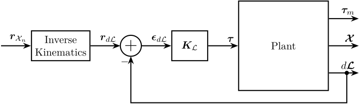
Figure 3: Control in the frame of the legs
2.2 Control in the Cartesian frame
From the relative displacement of each leg \(d\bm{\mathcal{L}}\), the pose of the nano-hexapod’s mobile platform \(\bm{\mathcal{X}_n}\) is estimated. It is then subtracted from reference pose of the nano-hexapod \(\bm{r}_{\mathcal{X}_n}\) to obtain the pose error \(\bm{\epsilon}_{\mathcal{X}_n}\). A diagonal controller \(\bm{K}_\mathcal{X}\) is used to generate forces and torques applied on the payload in a frame attached to the nano-hexapod’s base. These forces are then converted to forces applied in each of the nano-hexapod’s actuators by the use of the Jacobian \(\bm{J}^{-T}\).
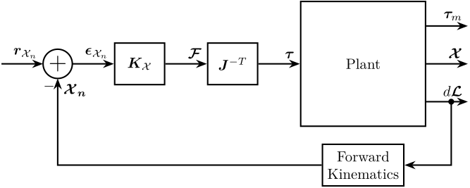
Figure 4: Control in the cartesian Frame (rotating frame attached to the nano-hexapod’s base)
3 Active Damping Architecture - Collocated Control (link)
From (Preumont 2018):
Active damping is very effective in reducing the settling time of transient disturbances and the effect of steady state disturbances near the resonance frequencies of the system; however, away from the resonances, the active damping is completely ineffective and leaves the closed-loop response essentially unchanged. Such low-gain controllers are often called Low Authority Controllers (LAC), because they modify the poles of the system only slightly.
Two very well known active damping techniques are Integral Force Feedback and Direct Velocity Feedback.
These two active damping techniques are collocated control techniques.
The active damping techniques are studied in this document.
3.1 Integral Force Feedback
In this active damping technique, the force sensors in each leg is used.
The controller \(\bm{K}_\text{IFF}\) is a diagonal matrix, each of its diagonal element consists of:
- an pure integrator
- a gain \(g\) that can be tuned to achieve a maximum damping
A lead-lag can also be used instead of a pure integrator.
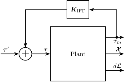
Figure 5: Integral Force Feedback
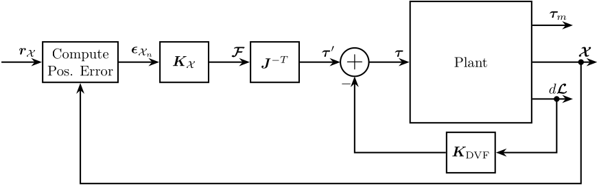
3.2 Direct Relative Velocity Feedback
The controller \(\bm{K}_\text{DVF}\) is a diagonal matrix. Each diagonal element consists of:
- a derivative action up to some frequency \(\omega_0\)
- a gain \(g\) that can be tuned to achieve a maximum damping

Figure 6: Direct Velocity Feedback
4 HAC-LAC Architectures (link)
Here we can combine Active Damping Techniques (Low authority control) with a tracking controller (high authority control). Usually, the low authority controller is designed first, and the high authority controller is designed based on the damped plant.
From (Preumont 2018):
The HAC/LAC approach consist of combining the two approached in a dual-loop control as shown in Figure 7. The inner loop uses a set of collocated actuator/sensor pairs for decentralized active damping with guaranteed stability ; the outer loop consists of a non-collocated HAC based on a model of the actively damped structure. This approach has the following advantages:
- The active damping extends outside the bandwidth of the HAC and reduces the settling time of the modes which are outsite the bandwidth
- The active damping makes it easier to gain-stabilize the modes outside the bandwidth of the output loop (improved gain margin)
- The larger damping of the modes within the controller bandwidth makes them more robust to the parmetric uncertainty (improved phase margin)
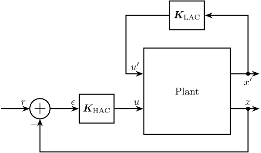
Figure 7: HAC-LAC Control Architecture
If there is only one input to the system, the HAC-LAC topology can be represented as depicted in Figure 8. Usually, the Low Authority Controller is first design, and then the High Authority Controller is designed based on the damped plant.
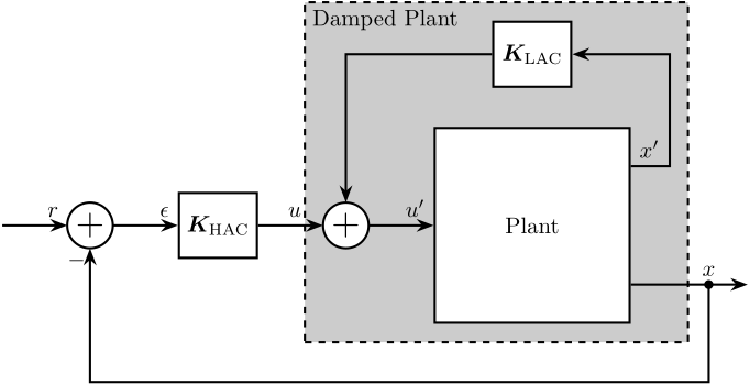
Figure 8: HAC-LAC Architecture with a system having only one input
4.1 HAC-LAC using IFF and Tracking control in the frame of the Legs
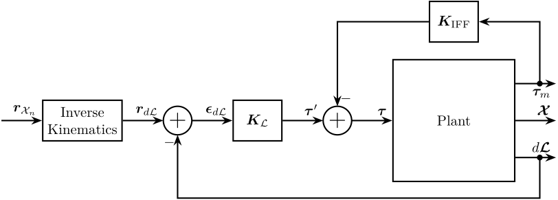
Figure 9: IFF + Control in the frame of the legs
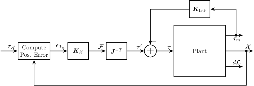
4.2 HAC-LAC using IFF and Tracking control in the Cartesian frame
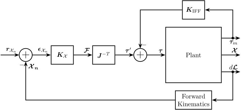
Figure 10: IFF + Control in the cartesian frame
4.3 HAC-LAC using IFF - the HAC controller is positioning the sample w.r.t. the granite in the task space
4.4 HAC-LAC using IFF - the HAC controller is positioning the sample w.r.t. the granite in the space of the legs

4.5 HAC-LAC using DVF - the HAC controller is positioning the sample w.r.t. the granite in the task space
4.6 HAC-LAC using DVF - the HAC controller is positioning the sample w.r.t. the granite in the space of the legs

5 Cascade Architectures (link)
The principle of Cascade control is shown in Figure 15 and explained as follow:
To follow two objectives with different properties in one control system, usually a hierarchy of two feedback loops is used in practice. This kind of control topology is called cascade control, which is used when there are several measurements and one prime control variable. Cascade control is implemented by nesting the control loops, as shown in Figure 15. The output control loop is called the primary loop, while the inner loop is called the secondary loop and is used to fulfill a secondary objective in the closed-loop system. – (Taghirad 2013)
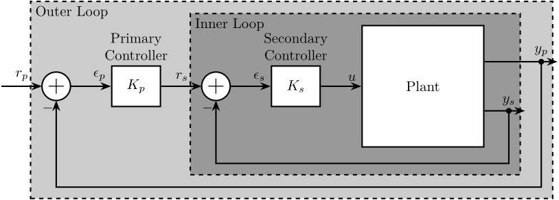
Figure 15: Cascade Control Architecture
This control topology seems adapted for the NASS, as indeed we have more inputs than outputs
In the NASS’s case:
- The primary objective is to position the sample with respect to the granite, thus the outer loop (and primary controller) should corresponds to a motion control loop
The inner loop can be composed of the system controlled with the HAC-LAC topology.
5.1 Cascade Control with HAC-LAC Inner Loop and Primary Controller in the task space
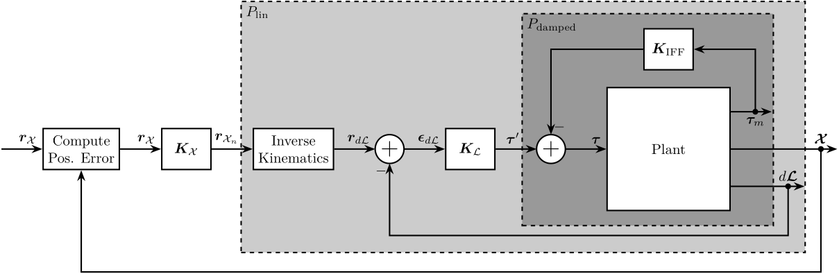
Figure 16: Cascaded Control consisting of (from inner to outer loop): IFF, Linearization Loop, Tracking Control in the frame of the Legs
5.2 Cascade Control with HAC-LAC Inner Loop and Primary Controller in the joint space
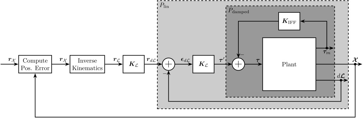
Figure 17: Cascaded Control consisting of (from inner to outer loop): IFF, Linearization Loop, Tracking Control in the Cartesian Frame
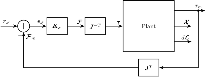
6 Force Control (link)
Signals:
- \(\bm{r}_\mathcal{F}\) is the wanted total force/torque to be applied to the payload
- \(\bm{\epsilon}_\mathcal{F}\) is the force/torque errors that should be applied to the payload
- \(\bm{\tau}\) is the force applied in each actuator
7 Other Control Architectures
7.1 Control to force the nano-hexapod to not do any vertical rotation
As the sample rotation around the vertical axis is not measure, the best we can do with the nano-hexapod is to not rotate around this same axis.
One way to do it is shown in Figure 19.
The controller \(\bm{K}_{R_z}\) is decomposed as shown in Figure 20.
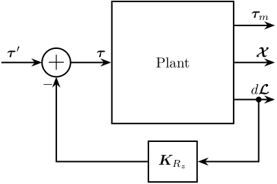
Figure 19: Figure caption
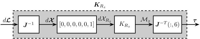
Figure 20: Figure caption