Modal Analysis - Measurement
Table of Contents
- 1. Instrumentation Used
- 2. Structure Preparation and Test Planning
- 3. Signal Processing
- 4. Force and Response signals
- 5. Frequency Response Functions and Coherence Results
- 6. Generation of a FRF matrix and a Coherence matrix from the measurements
- 7. Plot showing the coherence of all the measurements
- 8. Solid Bodies considered for further analysis
- 9. Note about the solid body assumption
- 10. Verification of the principle of reciprocity
The goal is to measure the dynamic of the Micro-Station and to extract Frequency Response Functions.
All the files (data and Matlab scripts) are accessible here.
1 Instrumentation Used
In order to perform to Modal Analysis and to obtain first a Response Model, the following devices are used:
- An acquisition system (OROS) with 24bits ADCs (figure 1)
- 3 tri-axis Accelerometers (figure 2) with parameters shown on table 1
- An Instrumented Hammer with various Tips (figure 3) (figure 4)
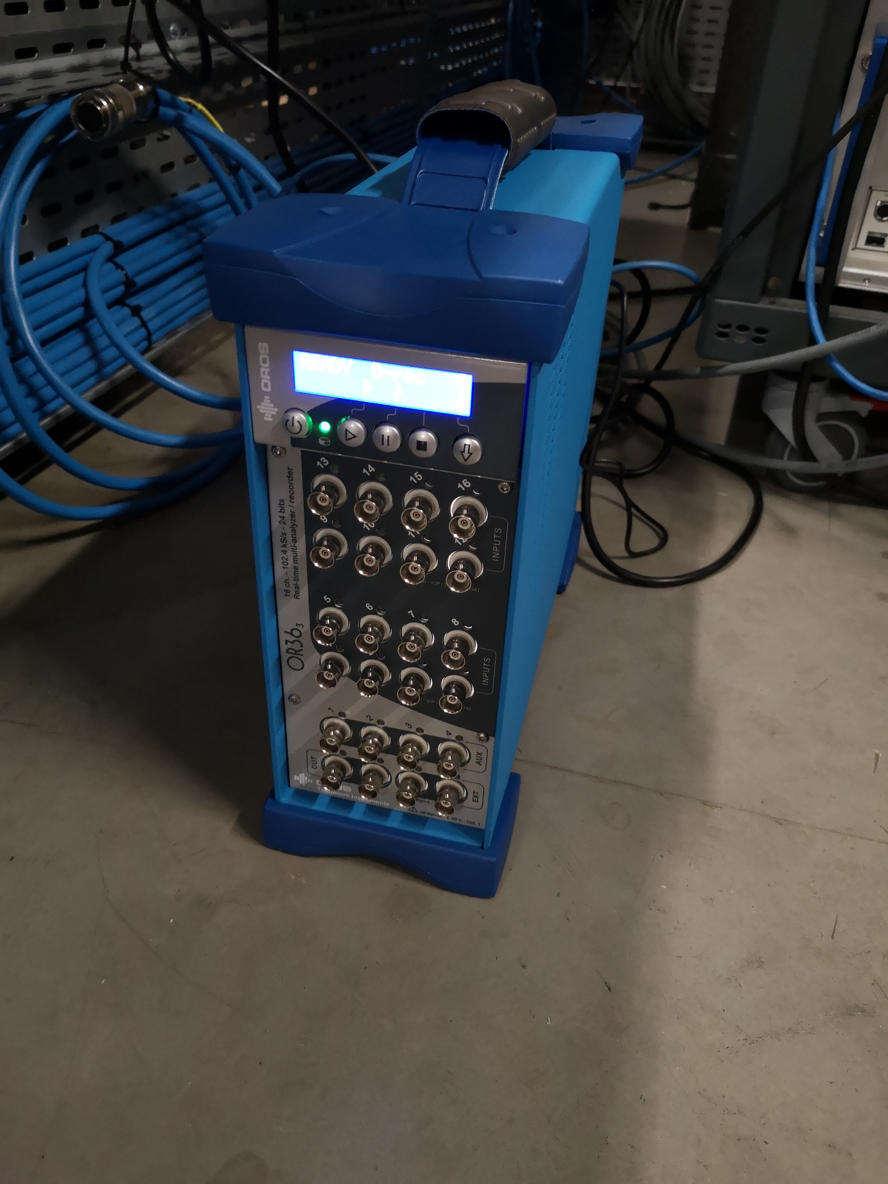
Figure 1: Acquisition system: OROS
The acquisition system permits to auto-range the inputs (probably using variable gain amplifiers) the obtain the maximum dynamic range. This is done before each measurement. Anti-aliasing filters are also included in the system.
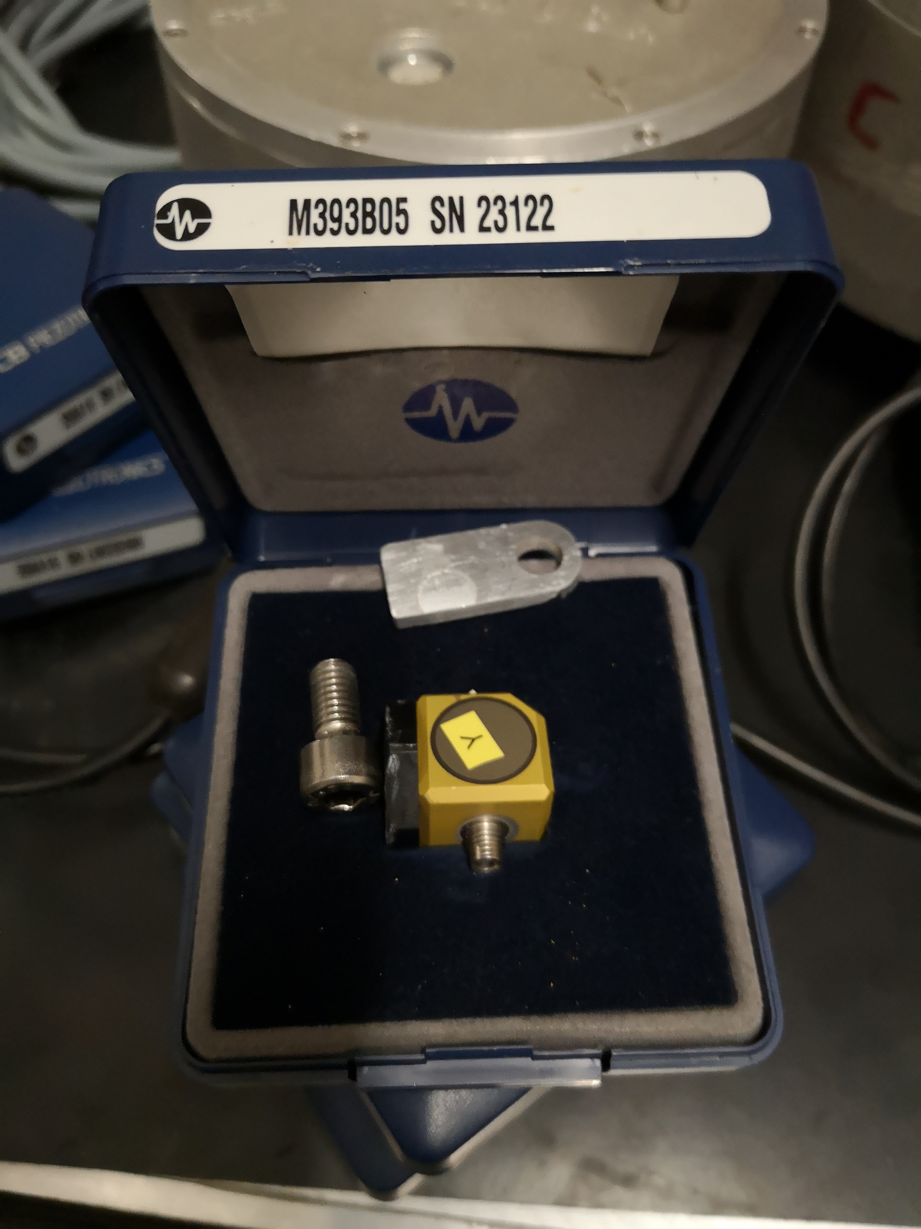
Figure 2: Accelerometer used: M393B05
| Sensitivity | 10V/g |
| Measurement Range | 0.5 g pk |
| Broadband Resolution | 0.000004 g rms |
| Frequency Range | 0.7 to 450Hz |
| Resonance Frequency | > 2.5kHz |
Tests have been conducted to determine the most suitable Hammer tip. This has been found that the softer tip gives the best results. It excites more the low frequency range where the coherence is low, the overall coherence was improved.
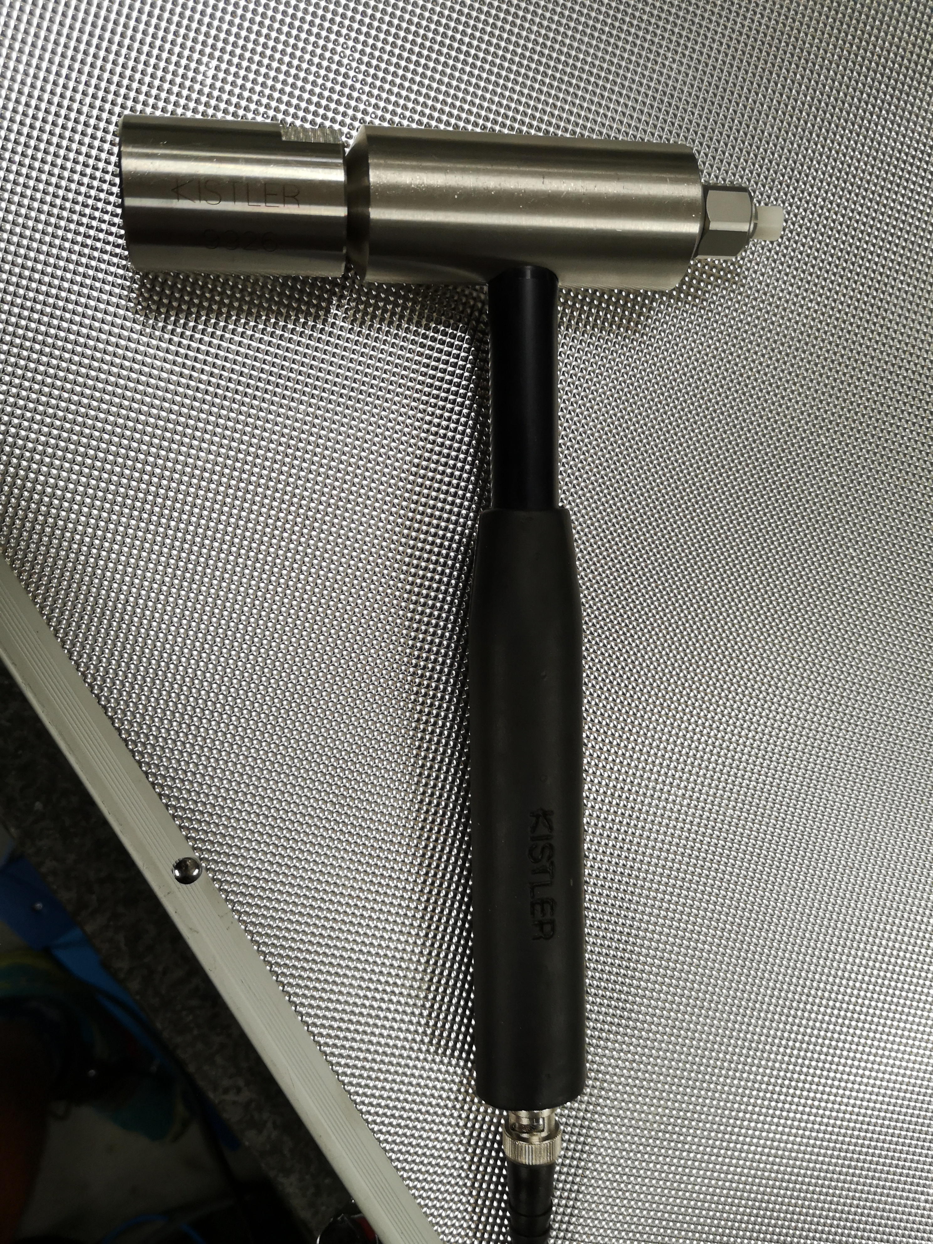
Figure 3: Instrumented Hammer
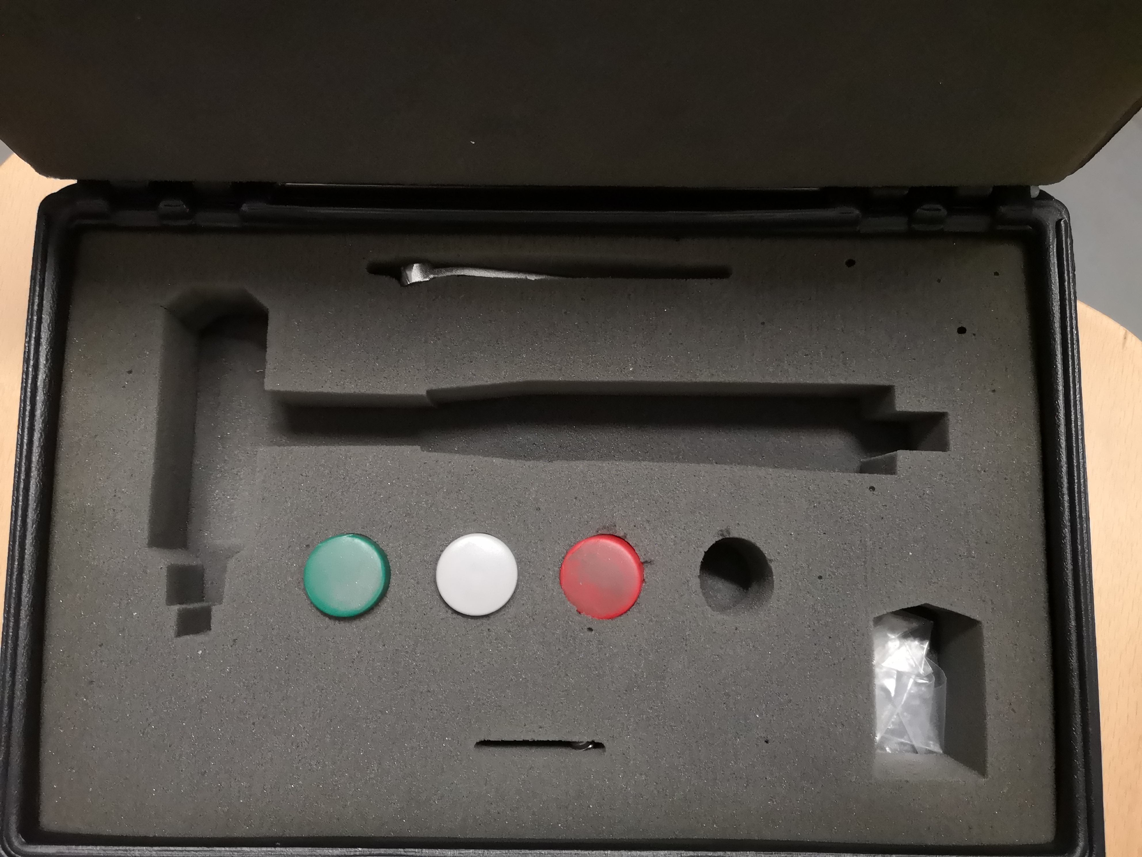
Figure 4: Hammer tips
The accelerometers are glued on the structure.
2 Structure Preparation and Test Planning
2.1 Structure Preparation
All the stages are turned ON. This is done for two reasons:
- Be closer to the real dynamic of the station in used
- If the control system of stages are turned OFF, this would results in very low frequency modes un-identifiable with the current setup, and this will also decouple the dynamics which would not be the case in practice
This is critical for the translation stage and the spindle as their is no stiffness in the free DOF (air-bearing for the spindle for instance).
The alternative would have been to mechanically block the stages with screws, but this may result in changing the modes.
The stages turned ON are:
- Translation Stage
- Tilt Stage
- Spindle and Slip-Ring
- Hexapod
The top part representing the NASS and the sample platform have been removed in order to reduce the complexity of the dynamics and also because this will be further added in the model inside Simscape.
All the stages are moved to their zero position (Ty, Ry, Rz, Slip-Ring, Hexapod).
All other elements have been remove from the granite such as another heavy positioning system.
2.2 Test Planing
The goal is to identify the full \(N \times N\) FRF matrix \(H\) (where \(N\) is the number of degree of freedom of the system):
\begin{equation} H_{jk} = \frac{X_j}{F_k} \end{equation}However, from only one column or one line of the matrix, we can compute the other terms thanks to the principle of reciprocity.
Either we choose to identify \(\frac{X_k}{F_i}\) or \(\frac{X_i}{F_k}\) for any chosen \(k\) and for \(i = 1,\ ...,\ N\).
We here choose to identify \(\frac{X_i}{F_k}\) for practical reasons:
- it is easier to glue the accelerometers on all the stages and excite only a one particular point than doing the opposite
The measurement thus consists of:
- always excite the structure at the same location with the Hammer
- Move the accelerometers to measure all the DOF of the structure
We will measured 3 columns (3 impacts location) in order to have some redundancy.
2.3 Location of the Accelerometers
4 tri-axis accelerometers are used for each solid body.
Only 2 could have been used as only 6DOF have to be measured, however, we have chosen to have some redundancy.
This could also help us identify measurement problems or flexible modes is present.
The position of the accelerometers are:
- 4 on the first granite
- 4 on the second granite (figure 5)
- 4 on top of the translation stage (figure 6)
- 4 on top of the tilt stage
- 3 on top of the spindle
- 4 on top of the hexapod (figure 7)
In total, 23 accelerometers are used: 69 DOFs are thus measured.
The position and orientation of all the accelerometers used are shown on figure 8.
The precise determination of the position of each accelerometer is done using the SolidWorks model (shown on figure 9).
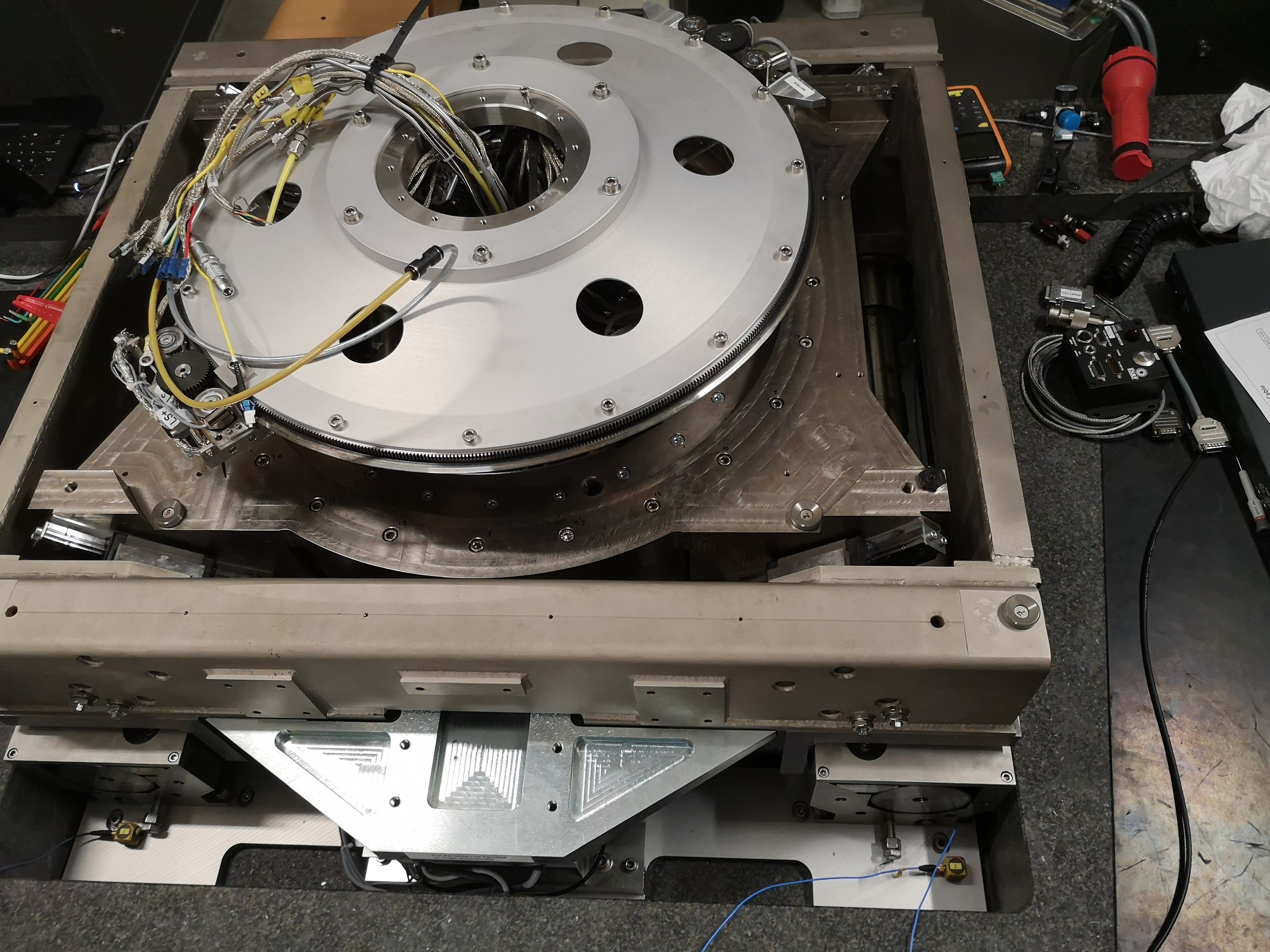
Figure 5: Accelerometers located on the top granite
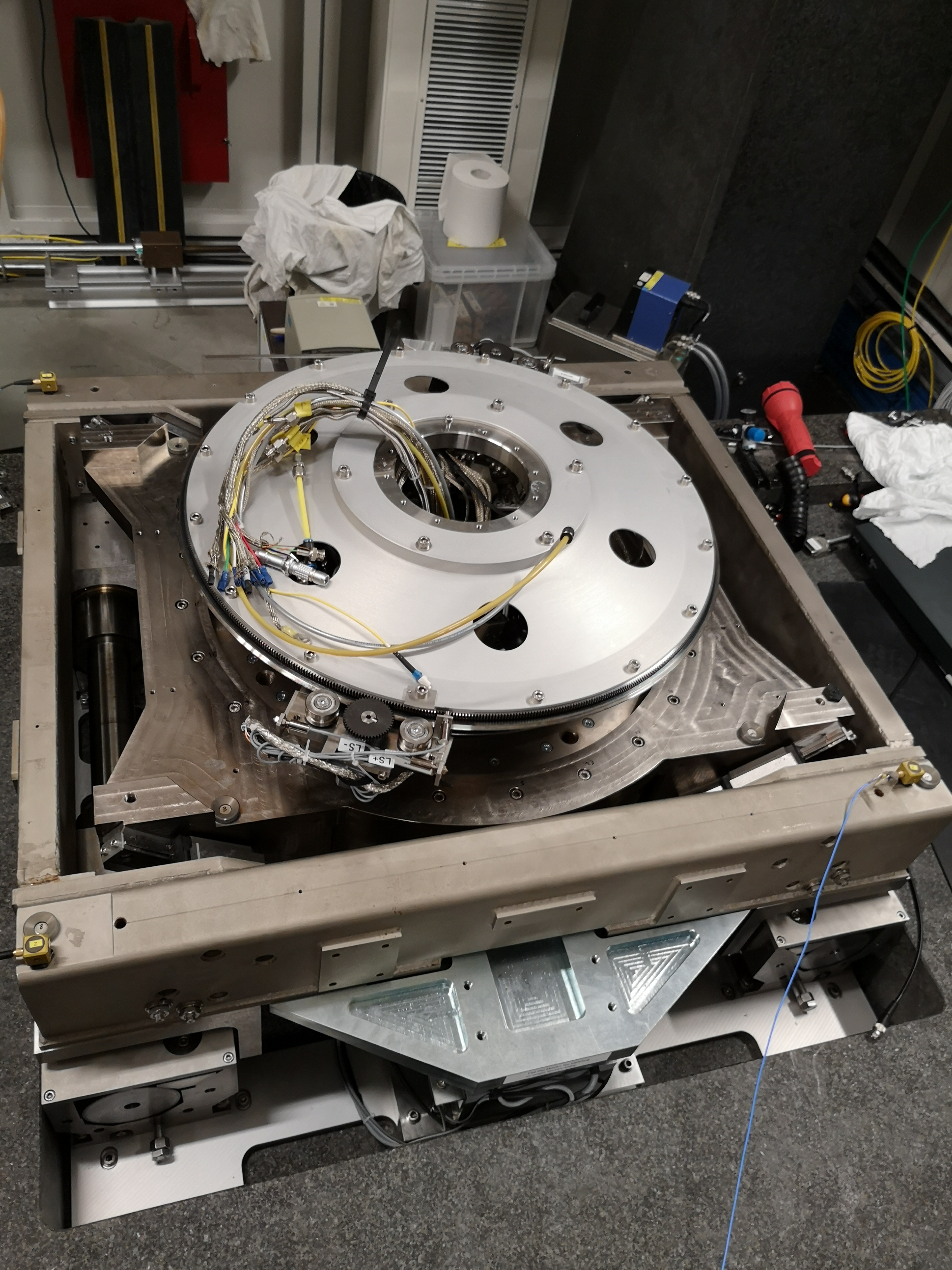
Figure 6: Accelerometers located on top of the translation stage
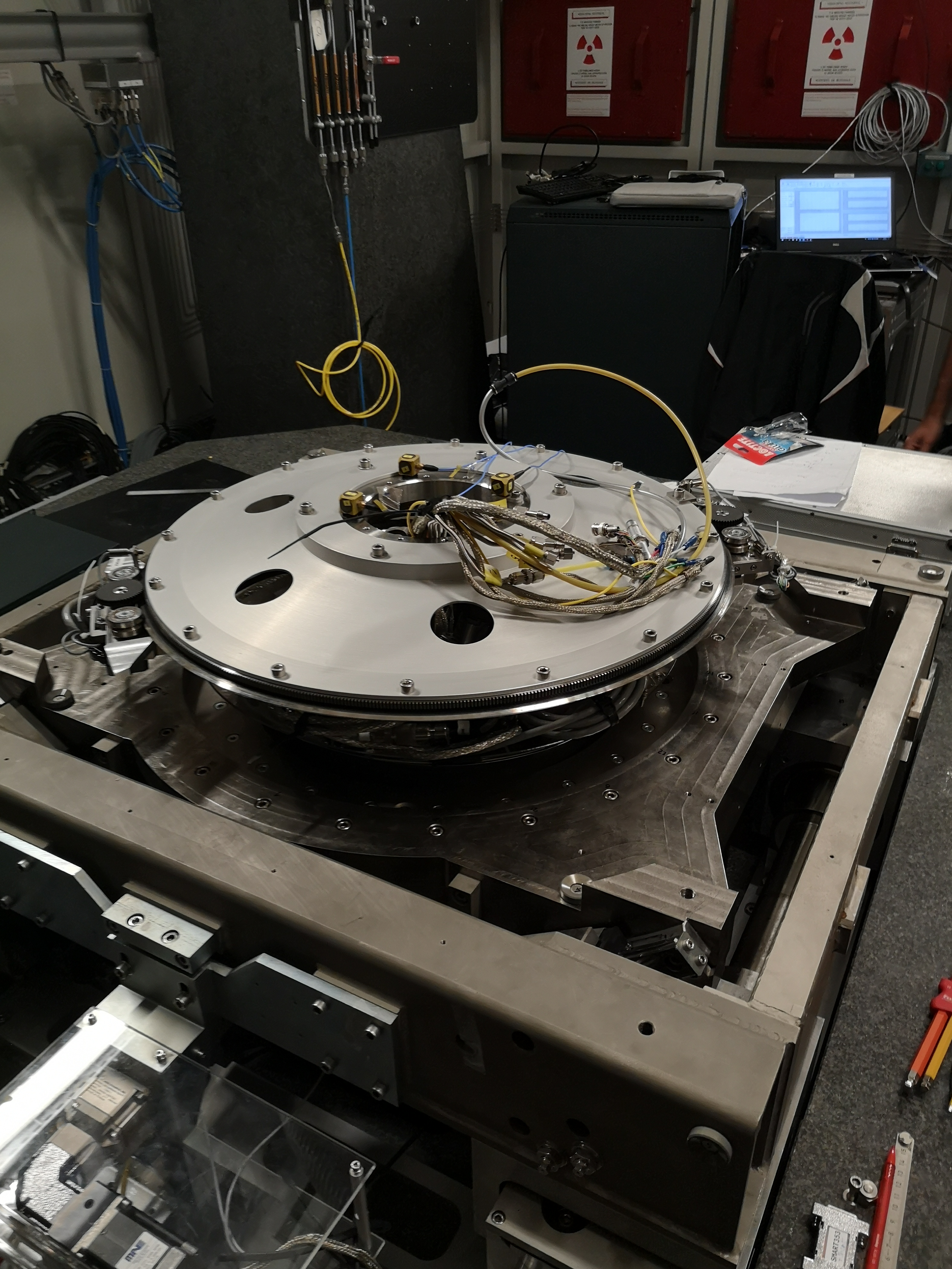
Figure 7: Accelerometers located on the Hexapod
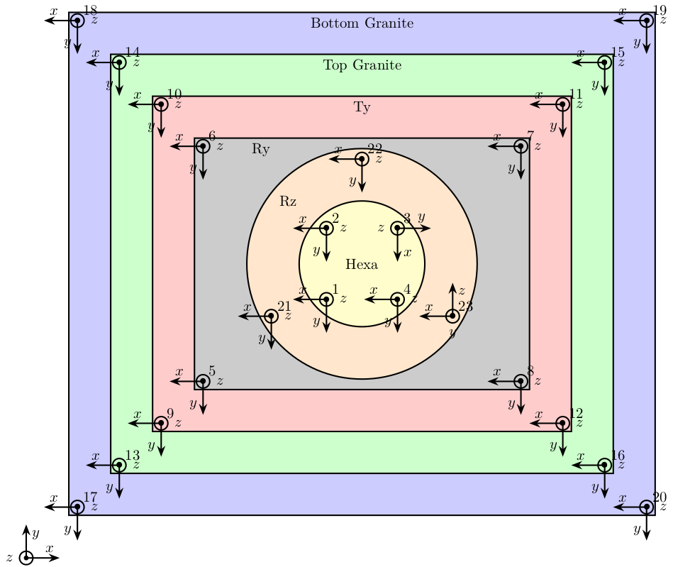
Figure 8: Position and orientation of the accelerometer used
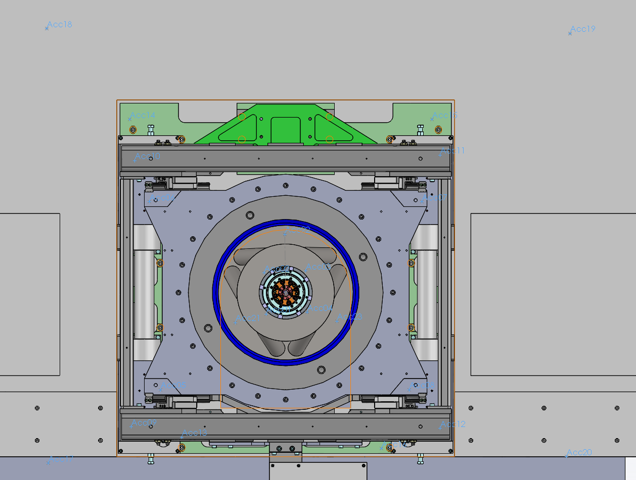
Figure 9: Position of the accelerometers using SolidWorks
The precise position of all the 23 accelerometer with respect to a frame located at the point of interest (located 270mm above the top platform of the hexapod) is shown below. The values are in meter.
They are contained in the mat/id31_nanostation.cfg file.
cat mat/id31_nanostation.cfg | grep NODES -A 23 | sed '/\s\+[0-9]\+/!d' | sed 's/\(.*\)\s\+0\s\+.\+/\1/' > mat/acc_pos.txt
We then import that on matlab, and sort them.
acc_pos = readtable('mat/acc_pos.txt', 'ReadVariableNames', false);
acc_pos = table2array(acc_pos(:, 1:4));
[~, i] = sort(acc_pos(:, 1));
acc_pos = acc_pos(i, 2:4);
The positions of the sensors relative to the point of interest are shown below (table 2).
| ID | x [mm] | y [mm] | z [mm] |
|---|---|---|---|
| 1 | -64 | -64 | -270 |
| 2 | -64 | 64 | -270 |
| 3 | 64 | 64 | -270 |
| 4 | 64 | -64 | -270 |
| 5 | -385 | -300 | -417 |
| 6 | -420 | 280 | -417 |
| 7 | 420 | 280 | -417 |
| 8 | 380 | -300 | -417 |
| 9 | -475 | -414 | -427 |
| 10 | -465 | 407 | -427 |
| 11 | 475 | 424 | -427 |
| 12 | 475 | -419 | -427 |
| 13 | -320 | -446 | -786 |
| 14 | -480 | 534 | -786 |
| 15 | 450 | 534 | -786 |
| 16 | 295 | -481 | -786 |
| 17 | -730 | -526 | -951 |
| 18 | -735 | 814 | -951 |
| 19 | 875 | 799 | -951 |
| 20 | 865 | -506 | -951 |
| 21 | -155 | -90 | -594 |
| 22 | 0 | 180 | -594 |
| 23 | 155 | -90 | -594 |
2.4 Hammer Impacts
Only 3 impact points are used.
The impact points are shown on figures 10, 11 and 12.
We chose this excitation point as it seems to excite all the modes in the frequency band of interest and because it provides good coherence for all the accelerometers.
Figure 10: Hammer Blow in the X direction
Figure 11: Hammer Blow in the Y direction
Figure 12: Hammer Blow in the Z direction
3 Signal Processing
3.1 Averaging
The measurements are averaged 10 times corresponding to 10 hammer impacts in order to reduce the effect of random noise. The parameters for the impact test are shown on table 3.
| Start Delay | -5% |
| Number of lines | 801 lines |
| Trigger Threshold | 300N |
| Trigger Hysteresis | 100mN |
| FRF Average | 10 |
3.2 Windowing
Windowing is used on the force and response signals.
A boxcar window (figure 13) is used for the force signal as once the impact on the structure is done, the measured signal is meaningless. The parameters are:
- Start: \(3\%\)
- Stop: \(7\%\)
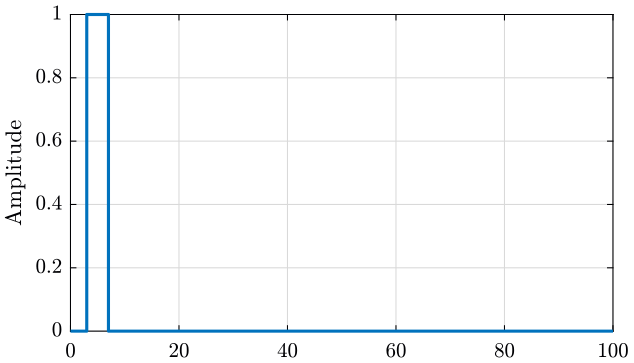
Figure 13: Window used for the force signal
An exponential window (figure 14) is used for the response signal as we are measuring transient signals and most of the information is located at the beginning of the signal. The parameters are:
- FlatTop:
- Start: \(3\%\)
- Stop: \(2.96\%\)
- Decreasing point:
- X: \(60.4\%\)
- Y: \(14.7\%\)
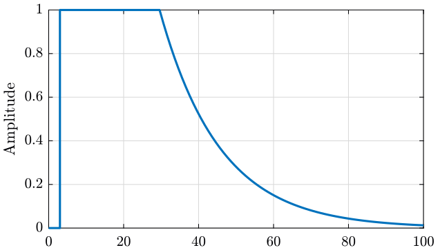
Figure 14: Window used for the response signals
4 Force and Response signals
Let's load some obtained data to look at the force and response signals.
meas1_raw = load('mat/meas_raw_1.mat');
4.1 Raw Force Data
The force input for the first measurement is shown on figure 15. We can see 10 impacts, one zoom on one impact is shown on figure 16.
The Fourier transform of the force is shown on figure 17. This has been obtained without any windowing.
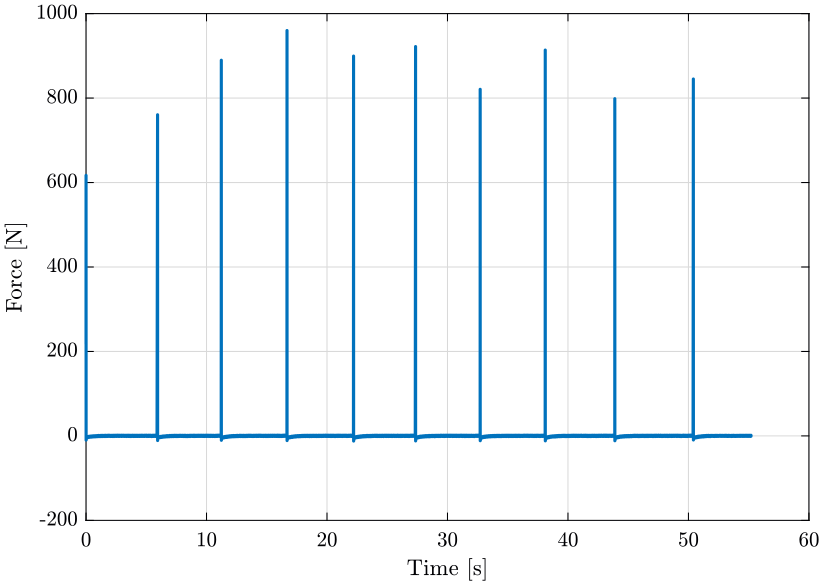
Figure 15: Raw Force Data from Hammer Blow
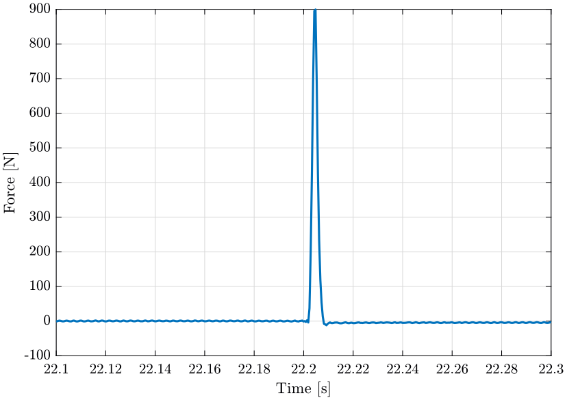
Figure 16: Raw Force Data from Hammer Blow - Zoom
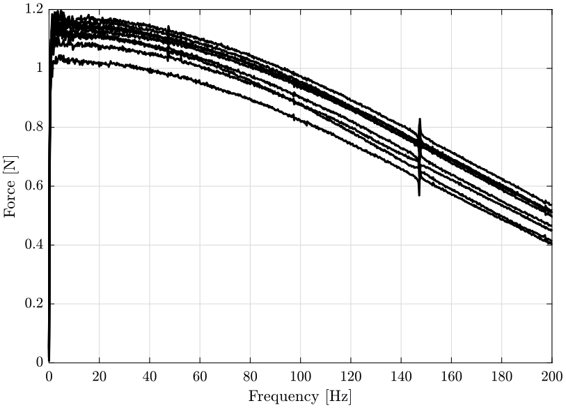
Figure 17: Fourier Transform of the 10 force impacts for the first measurement
4.2 Raw Response Data
The response signal for the first measurement is shown on figure 18. One zoom on one response is shown on figure 19.
The Fourier transform of the response signals is shown on figure 20. This has been obtained without any windowing.
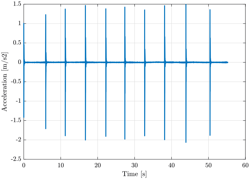
Figure 18: Raw Acceleration Data from Accelerometer
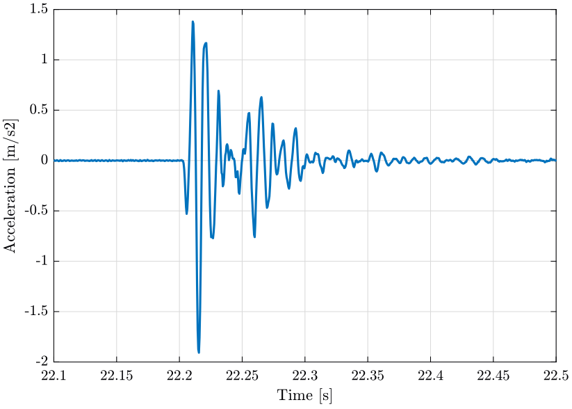
Figure 19: Raw Acceleration Data from Accelerometer - Zoom
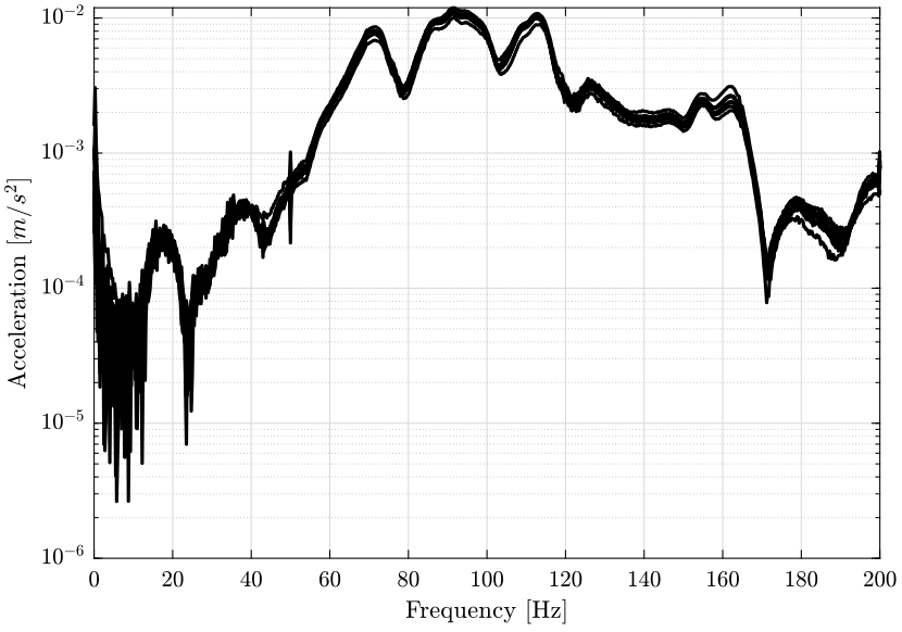
Figure 20: Fourier transform of the measured response signals
4.3 Computation of one Frequency Response Function
Now that we have obtained the Fourier transform of both the force input and the response signal, we can compute the Frequency Response Function from the force to the acceleration.
We then compare the result obtained with the FRF computed by the modal software (figure 21).
The slight difference can probably be explained by the use of windows.
In the following analysis, FRF computed from the software will be used.
meas1 = load('mat/meas_frf_coh_1.mat');
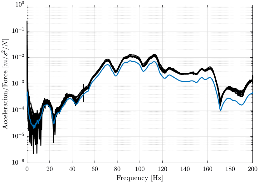
Figure 21: Comparison of the computed FRF from the Fourier transform and using the modal software
5 Frequency Response Functions and Coherence Results
Let's see one computed Frequency Response Function and one coherence in order to attest the quality of the measurement.
First, we load the data.
meas1 = load('mat/meas_frf_coh_1.mat');
And we plot on figure 22 the frequency response function from the force applied in the \(X\) direction at the location of the accelerometer number 11 to the acceleration in the \(X\) direction as measured by the first accelerometer located on the top platform of the hexapod.
The coherence associated is shown on figure 22.
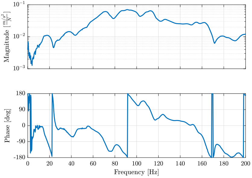
Figure 22: Example of one measured FRF
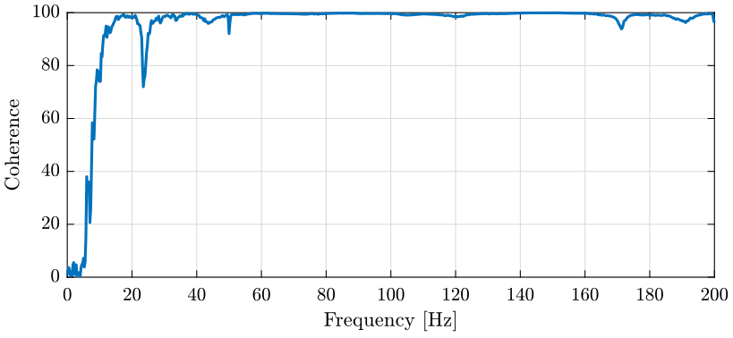
Figure 23: Example of one measured Coherence
6 Generation of a FRF matrix and a Coherence matrix from the measurements
We want here to combine all the Frequency Response Functions measured into one big array called the Frequency Response Matrix.
The frequency response matrix is an \(n \times p \times q\):
- \(n\) is the number of measurements: \(23 \times 3\) (23 accelerometers measuring 3 directions each)
- \(p\) is the number of excitation inputs: \(3\)
- \(q\) is the number of frequency points \(\omega_i\)
Thus, the FRF matrix is an \(69 \times 3 \times 801\) matrix. We do the same thing for the coherence matrix.
For each frequency point \(\omega_i\), we obtain a 2D matrix:
\begin{equation} \text{FRF}(\omega_i) = \begin{bmatrix} \frac{D_{1_x}}{F_x}(\omega_i) & \frac{D_{1_x}}{F_y}(\omega_i) & \frac{D_{1_x}}{F_z}(\omega_i) \\ \frac{D_{1_y}}{F_x}(\omega_i) & \frac{D_{1_y}}{F_y}(\omega_i) & \frac{D_{1_y}}{F_z}(\omega_i) \\ \frac{D_{1_z}}{F_x}(\omega_i) & \frac{D_{1_z}}{F_y}(\omega_i) & \frac{D_{1_z}}{F_z}(\omega_i) \\ \frac{D_{2_x}}{F_x}(\omega_i) & \frac{D_{2_x}}{F_y}(\omega_i) & \frac{D_{2_x}}{F_z}(\omega_i) \\ \vdots & \vdots & \vdots \\ \frac{D_{23_z}}{F_x}(\omega_i) & \frac{D_{23_z}}{F_y}(\omega_i) & \frac{D_{23_z}}{F_z}(\omega_i) \\ \end{bmatrix} \end{equation}We generate such FRF matrix from the measurements using the following script.
n_meas = 24;
n_acc = 23;

dirs = 'XYZ';

% Number of Accelerometer * DOF for each acccelerometer / Number of excitation / frequency points
FRFs = zeros(3*n_acc, 3, 801);
COHs = zeros(3*n_acc, 3, 801);

% Loop through measurements
for i = 1:n_meas
  % Load the measurement file
  meas = load(sprintf('mat/meas_frf_coh_%i.mat', i));

  % First: determine what is the exitation (direction and sign)
  exc_dir = meas.FFT1_AvXSpc_2_1_RMS_RfName(end);
  exc_sign = meas.FFT1_AvXSpc_2_1_RMS_RfName(end-1);
  % Determine what is the correct excitation sign
  exc_factor = str2num([exc_sign, '1']);
  if exc_dir ~= 'Z'
    exc_factor = exc_factor*(-1);
  end

  % Then: loop through the nine measurements and store them at the correct location
  for j = 2:10
    % Determine what is the accelerometer and direction
    [indices_acc_i] = strfind(meas.(sprintf('FFT1_H1_%i_1_RpName', j)), '.');
    acc_i = str2num(meas.(sprintf('FFT1_H1_%i_1_RpName', j))(indices_acc_i(1)+1:indices_acc_i(2)-1));

    meas_dir  = meas.(sprintf('FFT1_H1_%i_1_RpName', j))(end);
    meas_sign = meas.(sprintf('FFT1_H1_%i_1_RpName', j))(end-1);
    % Determine what is the correct measurement sign
    meas_factor = str2num([meas_sign, '1']);
    if meas_dir ~= 'Z'
      meas_factor = meas_factor*(-1);
    end

    FRFs(find(dirs==meas_dir)+3*(acc_i-1), find(dirs==exc_dir), :) = exc_factor*meas_factor*meas.(sprintf('FFT1_H1_%i_1_Y_ReIm', j));
    COHs(find(dirs==meas_dir)+3*(acc_i-1), find(dirs==exc_dir), :) = meas.(sprintf('FFT1_Coh_%i_1_RMS_Y_Val', j));
  end
end
freqs = meas.FFT1_Coh_10_1_RMS_X_Val;
And we save the obtained FRF matrix and Coherence matrix in a .mat file.
save('./mat/frf_coh_matrices.mat', 'FRFs', 'COHs', 'freqs');
7 Plot showing the coherence of all the measurements
Now that we have defined a Coherence matrix, we can plot each of its elements to have an idea of the overall coherence and thus, quality of the measurement. The result is shown on figure 24.
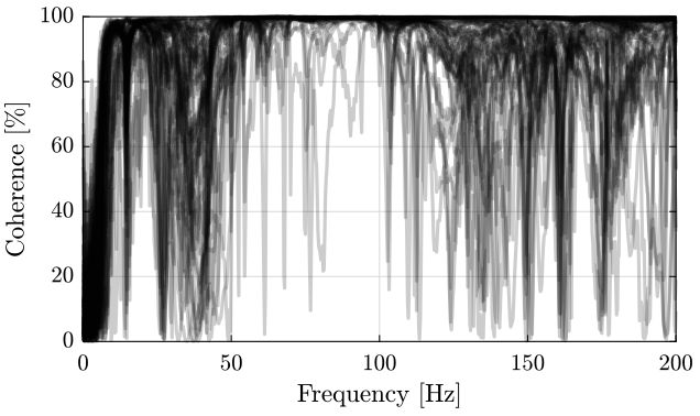
Figure 24: Plot of the coherence of all the measurements
8 Solid Bodies considered for further analysis
We consider the following solid bodies for further analysis:
- Bottom Granite
- Top Granite
- Translation Stage
- Tilt Stage
- Spindle
- Hexapod
We create a matlab structure solids that contains the accelerometers ID connected to each solid bodies (as shown on figure 8).
solids = {};
solids.gbot = [17, 18, 19, 20];
solids.gtop = [13, 14, 15, 16];
solids.ty   = [9, 10, 11, 12];
solids.ry   = [5, 6, 7, 8];
solids.rz   = [21, 22, 23];
solids.hexa = [1, 2, 3, 4];

solid_names = fields(solids);
Finally, we save that into a .mat file.
save('mat/geometry.mat', 'solids', 'solid_names', 'acc_pos');
9 Note about the solid body assumption
If we measure the motion of a rigid body along a direction \(\vec{x}\) using 2 sensors that are co-linear with the same direction \(\vec{x}\) (\(\vec{p}_2 = \vec{p}_1 + \alpha \vec{x}\)), they will measured the same quantity.
This is illustrated on figure 25.
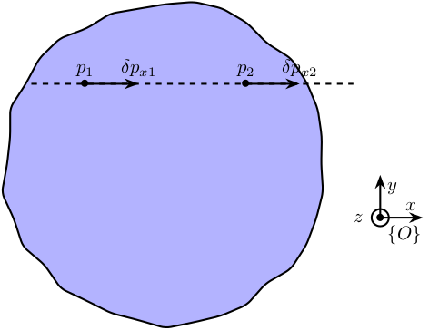
Figure 25: Aligned measurement of the motion of a solid body
The motion of the rigid body of figure 25 is defined by its displacement \(\delta p\) and rotation \(\vec{\Omega}\) with respect to the reference frame \(\{O\}\).
The motions at points \(1\) and \(2\) are:
\begin{align*} \delta p_1 &= \delta p + \Omega \times p_1 \\ \delta p_2 &= \delta p + \Omega \times p_2 \end{align*}Taking only the \(x\) direction:
\begin{align*} \delta p_{x1} &= \delta p_x + \Omega_y p_{z1} - \Omega_z p_{y1} \\ \delta p_{x2} &= \delta p_x + \Omega_y p_{z2} - \Omega_z p_{y2} \end{align*}However, we have \(p_{1y} = p_{2y}\) and \(p_{1z} = p_{2z}\) because of the co-linearity of the two sensors in the \(x\) direction, and thus we obtain
\begin{equation} \delta p_{x1} = \delta p_{x2} \end{equation}Two sensors that are measuring the motion of a rigid body in the direction of the line linking the two sensors should measure the same quantity.
We can verify that the rigid body assumption is correct by comparing the measurement of the sensors.
From the table 2, we can guess which sensors will give the same results in the X and Y directions.
Comparison of such measurements in the X direction is shown on figure 26 and in the Y direction on figure 27.
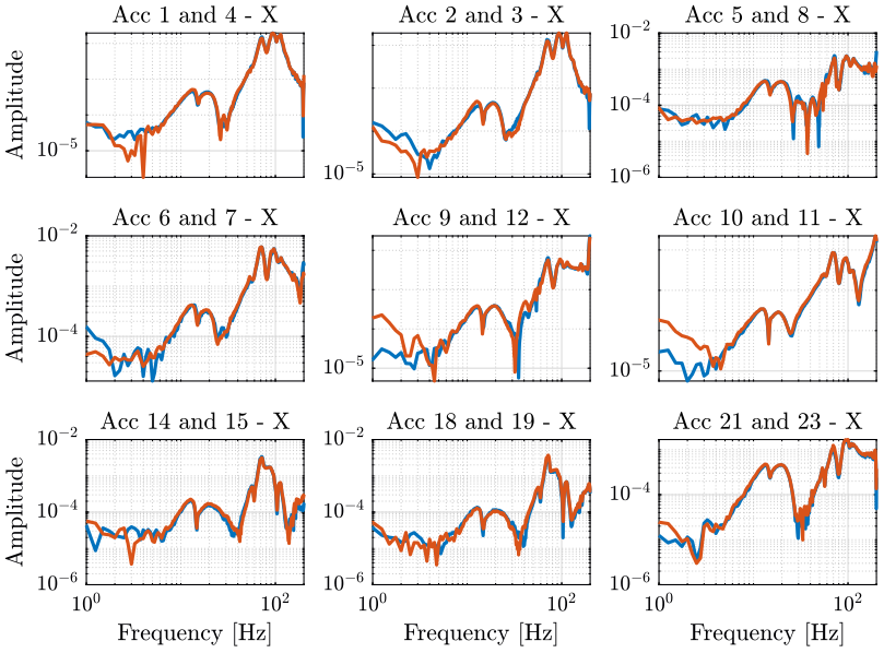
Figure 26: Compare accelerometers align in the X direction
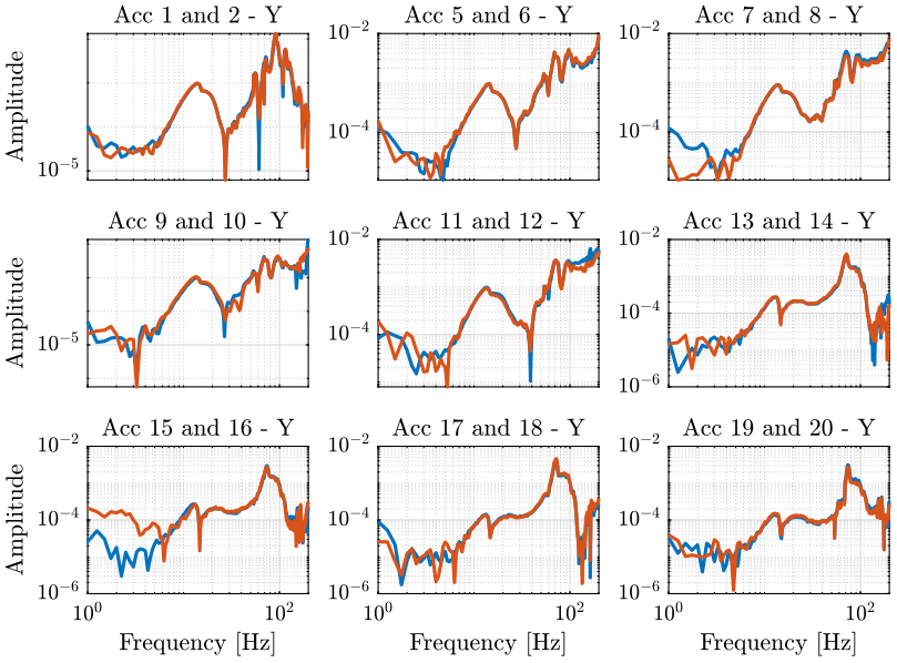
Figure 27: Compare accelerometers align in the Y direction
From the two figures above, we are more confident about the rigid body assumption in the frequency band of interest.
10 Verification of the principle of reciprocity
Because we expect our system to follow the principle of reciprocity. That is to say the response \(X_j\) at some degree of freedom \(j\) due to a force \(F_k\) applied on DOF \(k\) should be the same as the response \(X_k\) due to a force \(F_j\): \[ H_{jk} = \frac{X_j}{F_k} = \frac{X_k}{F_j} = H_{kj} \]
This comes from the fact that we expect to have symmetric mass, stiffness and damping matrices.
In order to access the quality of the data and the validity of the measured FRF, we then check that the reciprocity between \(H_{jk}\) and \(H_{kj}\) is of an acceptable level.
We can verify this reciprocity using 3 different pairs of response/force.
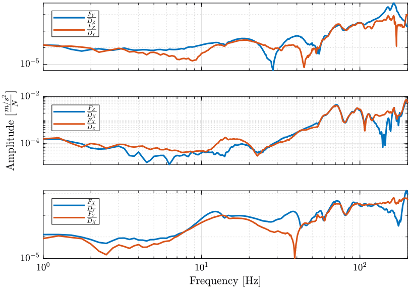
Figure 28: Verification of the principle of reciprocity
From figure 28, it seems that the principle of reciprocity is valid from 50Hz to 100Hz. Above that, the difference between the two could be due to:
- rotational DOFs? Local flexibility?
Below, it could be due to:
- not exciting and measuring the same DOF
One should note here that the excitation is not applied on the same DOF as the measured response. This could be seen on figures 10, 11 and 12 that show the excitation points, and on figure 6 where the accelerometer on the bottom left shows the one used for the principle of reciprocity validation above. Thus, technically we cannot verify the principle of reciprocity here.
As it is usually very important to measure point response \(\frac{X_j}{F_j}\), that is to say exciting and measuring the same DOF, should the measurements be redone? On the modal software that is used to extract modal parameters, it is suppose that we are exciting the exact same DOF as the one measured by the accelerometer 11. As is it not the case in practice, could this induce large errors in the modal model?