Modal Analysis - Processing of FRF
Table of Contents
- 1. Importation of measured FRF curves
- 2. From accelerometer DOFs to solid body DOFs - Mathematics
- 3. What reference frame to choose?
- 4. FRF expressed in a common frame
- 4.1. From accelerometer DOFs to solid body DOFs - Matlab Implementation
- 4.2. Analysis of some FRF in the global coordinates
- 4.3. Comparison of the relative motion of solid bodies
- 4.4. Verify that we find the original FRF from the FRF in the global coordinates
- 4.5. Saving of the FRF expressed in the global coordinates
- 5. FRF expressed in a frame centered at the CoM of each solid body
The measurements have been conducted and we have computed the \(n \times p \times q\) Frequency Response Functions Matrix with:
- \(n\): the number of measurements: \(23 \times 3 = 69\) (23 accelerometers measuring 3 directions each)
- \(p\): the number of excitation inputs: \(3\)
- \(q\): the number of frequency points \(\omega_i\)
However, in our model, we only consider 6 solid bodies, namely:
- Bottom Granite
- Top Granite
- Translation Stage
- Tilt Stage
- Spindle
- Hexapod
Thus, we are only interested in \(6 \times 6 = 36\) degrees of freedom.
We here process the FRF matrix to go from the 69 measured DOFs to the wanted 36 DOFs.
All the files (data and Matlab scripts) are accessible here.
1 Importation of measured FRF curves
We load the measured FRF and Coherence matrices. We also load the geometric parameters of the station: solid bodies considered and the position of the accelerometers.
load('mat/frf_coh_matrices.mat', 'FRFs', 'COHs', 'freqs');
load('mat/geometry.mat', 'solids', 'solid_names', 'acc_pos');
2 From accelerometer DOFs to solid body DOFs - Mathematics
Let's consider the schematic shown on figure 1 where we are measuring the motion of a (supposed) solid body at 4 distinct points in x-y-z.
The goal here is to link these \(4 \times 3 = 12\) measurements to the 6 DOFs of the solid body expressed in the frame \(\{O\}\).
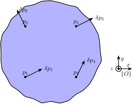
Figure 1: Schematic of the measured motions of a solid body
We consider the motion of the rigid body defined by its displacement \(\delta p\) and rotation \(\vec{\Omega}\) with respect to the reference frame \(\{O\}\).
From the figure 1, we can write:
\begin{align*} \delta p_1 &= \delta p + \delta\Omega p_1\\ \delta p_2 &= \delta p + \delta\Omega p_2\\ \delta p_3 &= \delta p + \delta\Omega p_3\\ \delta p_4 &= \delta p + \delta\Omega p_4 \end{align*}With
\begin{equation} \delta\Omega = \begin{bmatrix} 0 & -\delta\Omega_z & \delta\Omega_y \\ \delta\Omega_z & 0 & -\delta\Omega_x \\ -\delta\Omega_y & \delta\Omega_x & 0 \end{bmatrix} \end{equation}We can rearrange the equations in a matrix form:
\begin{equation} \left[\begin{array}{ccc|ccc} 1 & 0 & 0 & 0 & p_{1z} & -p_{1y} \\ 0 & 1 & 0 & -p_{1z} & 0 & p_{1x} \\ 0 & 0 & 1 & p_{1y} & -p_{1x} & 0 \\ \hline & \vdots & & & \vdots & \\ \hline 1 & 0 & 0 & 0 & p_{4z} & -p_{4y} \\ 0 & 1 & 0 & -p_{4z} & 0 & p_{4x} \\ 0 & 0 & 1 & p_{4y} & -p_{4x} & 0 \end{array}\right] \begin{bmatrix} \delta p_x \\ \delta p_y \\ \delta p_z \\ \hline \delta\Omega_x \\ \delta\Omega_y \\ \delta\Omega_z \end{bmatrix} = \begin{bmatrix} \delta p_{1x} \\ \delta p_{1y} \\ \delta p_{1z} \\\hline \vdots \\\hline \delta p_{4x} \\ \delta p_{4y} \\ \delta p_{4z} \end{bmatrix} \end{equation}and then we obtain the velocity and rotation of the solid in the wanted frame \(\{O\}\):
\begin{equation} \begin{bmatrix} \delta p_x \\ \delta p_y \\ \delta p_z \\ \hline \delta\Omega_x \\ \delta\Omega_y \\ \delta\Omega_z \end{bmatrix} = \left[\begin{array}{ccc|ccc} 1 & 0 & 0 & 0 & p_{1z} & -p_{1y} \\ 0 & 1 & 0 & -p_{1z} & 0 & p_{1x} \\ 0 & 0 & 1 & p_{1y} & -p_{1x} & 0 \\ \hline & \vdots & & & \vdots & \\ \hline 1 & 0 & 0 & 0 & p_{4z} & -p_{4y} \\ 0 & 1 & 0 & -p_{4z} & 0 & p_{4x} \\ 0 & 0 & 1 & p_{4y} & -p_{4x} & 0 \end{array}\right]^{-1} \begin{bmatrix} \delta p_{1x} \\ \delta p_{1y} \\ \delta p_{1z} \\\hline \vdots \\\hline \delta p_{4x} \\ \delta p_{4y} \\ \delta p_{4z} \end{bmatrix} \label{eq:determine_global_disp} \end{equation}Using equation \eqref{eq:determine_global_disp}, we can determine the motion of the solid body expressed in a chosen frame \(\{O\}\) using the accelerometers attached to it. The inversion is equivalent to resolving a mean square problem.
3 What reference frame to choose?
The question we wish here to answer is how to choose the reference frame \(\{O\}\) in which the DOFs of the solid bodies are defined.
The possibles choices are:
- One frame for each solid body which is located at its center of mass
- One common frame, for instance located at the point of interest (\(270mm\) above the Hexapod)
- Base located at the joint position: this is where we want to see the motion and estimate stiffness
| Chosen Frame | Advantages | Disadvantages |
|---|---|---|
| Frames at CoM | Physically, it makes more sense | How to compare the motion of the solid bodies? |
| Common Frame | We can compare the motion of each solid body | Small \(\theta_{x, y}\) may result in large \(T_{x, y}\) |
| Frames at joint position | Directly gives which joint direction can be blocked | How to choose the joint position? |
The choice of the frame depends of what we want to do with the data.
One of the goals is to compare the motion of each solid body to see which relative DOFs between solid bodies can be neglected, that is to say, which joint between solid bodies can be regarded as perfect (and this in all the frequency range of interest). Ideally, we would like to have the same number of degrees of freedom than the number of identified modes.
In the next sections, we will express the FRF matrix in the different frames.
4 FRF expressed in a common frame
4.1 From accelerometer DOFs to solid body DOFs - Matlab Implementation
First, we initialize a new FRF matrix FRFs_O which is an \(n \times p \times q\) with:
- \(n\) is the number of DOFs of the considered 6 solid-bodies: \(6 \times 6 = 36\)
- \(p\) is the number of excitation inputs: \(3\)
- \(q\) is the number of frequency points \(\omega_i\)
For each frequency point \(\omega_i\), the FRF matrix FRFs_O is a \(n\times p\) matrix:
where \(D_i\) corresponds to the solid body number i.
Then, as we know the positions of the accelerometers on each solid body, and we have the response of those accelerometers, we can use the equations derived in the previous section to determine the response of each solid body expressed in the frame \(\{O\}\).
FRFs_O = zeros(length(solid_names)*6, 3, 801);

for solid_i = 1:length(solid_names)
  solids_i = solids.(solid_names{solid_i});

  A = zeros(3*length(solids_i), 6);
  for i = 1:length(solids_i)
    acc_i = solids_i(i);

    A(3*(i-1)+1:3*i, 1:3) = eye(3);
    A(3*(i-1)+1:3*i, 4:6) = [ 0                  acc_pos(acc_i, 3) -acc_pos(acc_i, 2) ;
                             -acc_pos(acc_i, 3)  0                  acc_pos(acc_i, 1) ;
                              acc_pos(acc_i, 2) -acc_pos(acc_i, 1)  0];
  end

  for exc_dir = 1:3
    FRFs_O((solid_i-1)*6+1:solid_i*6, exc_dir, :) = A\squeeze(FRFs((solids_i(1)-1)*3+1:solids_i(end)*3, exc_dir, :));
  end
end
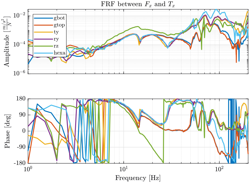
4.2 Analysis of some FRF in the global coordinates
4.3 Comparison of the relative motion of solid bodies
Now that the motion of all the solid bodies are expressed in the same frame, we should be able to compare them. This can be used to determine what joints direction between two solid bodies is stiff enough that we can fix this DoF. This could help reduce the order of the model and simplify the extraction of the model parameters from the measurements.
We decide to plot the "normalized relative motion" between solid bodies \(i\) and \(j\): \[ 0 < \Delta_{ij, x} = \frac{\left| |D_{i,x}| - |D_{j,x}| \right|}{|D_{i,x}| + |D_{j,x}|} < 1 \]
Then, if \(\Delta_{ij,x} \ll 1\) in the frequency band of interest, we have that \(D_{ix} \approx D_{jx}\) and we can neglect that DOF between the two solid bodies \(i\) and \(j\).
This normalized relative motion is shown on figure 4 for all the directions and for all the adjacent pair of solid bodies.
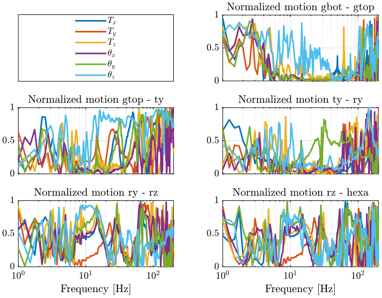
Figure 4: Relative motion between each stage
Can we really compare the motion of two solid bodies from Frequency Response Functions that clearly depends on the excitation point and direction? The relative motion of two solid bodies may be negligible when exciting the structure at on point and but at another point.
4.4 Verify that we find the original FRF from the FRF in the global coordinates
We have computed the Frequency Response Functions Matrix FRFs_O representing the response of the 6 solid bodies in their 6 DOFs with respect to the frame \(\{O\}\).
From the response of one body in its 6 DOFs, we should be able to compute the FRF of each of its accelerometer fixed to it during the measurement, supposing that the stage is a solid body.
We can then compare the result with the original measurements. This will help us to determine if:
- the previous inversion used is correct
- the solid body assumption is correct in the frequency band of interest
From the translation \(\delta p\) and rotation \(\delta \Omega\) of a solid body and the positions \(p_i\) of the accelerometers attached to it, we can compute the response that would have been measured by the accelerometers using the following formula:
\begin{align*} \delta p_1 &= \delta p + \delta\Omega p_1\\ \delta p_2 &= \delta p + \delta\Omega p_2\\ \delta p_3 &= \delta p + \delta\Omega p_3\\ \delta p_4 &= \delta p + \delta\Omega p_4 \end{align*}
Thus, we can obtain the FRF matrix FRFs_A that gives the responses of the accelerometers to the forces applied by the hammer.
It is implemented in matlab as follow:
FRFs_A = zeros(size(FRFs));

% For each excitation direction
for exc_dir = 1:3
  % For each solid
  for solid_i = 1:length(solid_names)
    v0 = squeeze(FRFs_O((solid_i-1)*6+1:(solid_i-1)*6+3, exc_dir, :));
    W0 = squeeze(FRFs_O((solid_i-1)*6+4:(solid_i-1)*6+6, exc_dir, :));

    % For each accelerometer attached to the current solid
    for acc_i = solids.(solid_names{solid_i})
      % We get the position of the accelerometer expressed in frame O
      pos = acc_pos(acc_i, :)';
      posX = [0 pos(3) -pos(2); -pos(3) 0 pos(1) ; pos(2) -pos(1) 0];

      FRFs_A(3*(acc_i-1)+1:3*(acc_i-1)+3, exc_dir, :) = v0 + posX*W0;
    end
  end
end
We then compare the original FRF measured for each accelerometer FRFs with the "recovered" FRF FRFs_A from the global FRF matrix in the common frame.
The FRF for the 4 accelerometers on the Hexapod are compared on figure 5. All the FRF are matching very well in all the frequency range displayed.
The FRF for accelerometers located on the translation stage are compared on figure 6. The FRF are matching well until 100Hz.
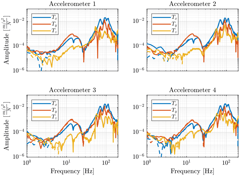
Figure 5: Comparison of the original FRF with the recovered ones - Hexapod
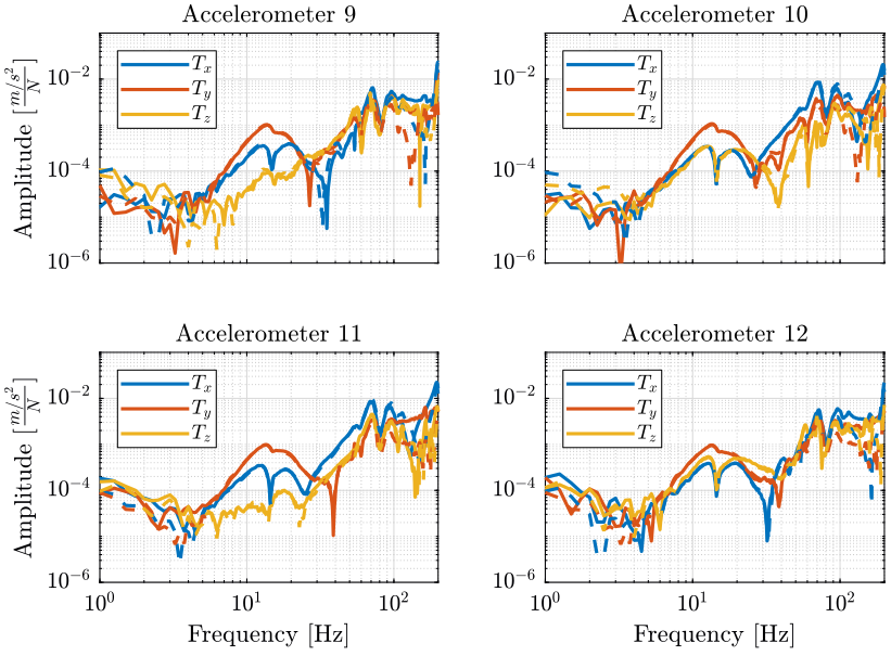
Figure 6: Comparison of the original FRF with the recovered ones - Ty
The reduction of the number of degrees of freedom from 69 (23 accelerometers with each 3DOF) to 36 (6 solid bodies with 6 DOF) seems to work well.
This confirms the fact that the stages are indeed behaving as a solid body in the frequency band of interest. This valid the fact that a multi-body model can be used to represent the dynamics of the micro-station.
4.5 Saving of the FRF expressed in the global coordinates
save('mat/frf_o.mat', 'FRFs_O');
5 FRF expressed in a frame centered at the CoM of each solid body
5.1 Center of Mass of each solid body
From solidworks, we can export the position of the center of mass of each solid body considered.
For that, we have to suppose density of the materials. We then process the exported file.
sed -e '1,/^Center of mass/ d' mat/1_granite_bot.txt | sed 3q | sed 's/^\s*\t*[XYZ] = \([-0-9.]*\)\r/\1/' >  mat/model_solidworks_com.txt
sed -e '1,/^Center of mass/ d' mat/2_granite_top.txt | sed 3q | sed 's/^\s*\t*[XYZ] = \([-0-9.]*\)\r/\1/' >> mat/model_solidworks_com.txt
sed -e '1,/^Center of mass/ d' mat/3_ty.txt          | sed 3q | sed 's/^\s*\t*[XYZ] = \([-0-9.]*\)\r/\1/' >> mat/model_solidworks_com.txt
sed -e '1,/^Center of mass/ d' mat/4_ry.txt          | sed 3q | sed 's/^\s*\t*[XYZ] = \([-0-9.]*\)\r/\1/' >> mat/model_solidworks_com.txt
sed -e '1,/^Center of mass/ d' mat/5_rz.txt          | sed 3q | sed 's/^\s*\t*[XYZ] = \([-0-9.]*\)\r/\1/' >> mat/model_solidworks_com.txt
sed -e '1,/^Center of mass/ d' mat/6_hexa.txt        | sed 3q | sed 's/^\s*\t*[XYZ] = \([-0-9.]*\)\r/\1/' >> mat/model_solidworks_com.txt
And we import the Center of mass on Matlab.
model_com = table2array(readtable('mat/model_solidworks_com.txt', 'ReadVariableNames', false));
model_com = reshape(model_com , [3, 6]);
| granite bot | granite top | ty | ry | rz | hexa | |
|---|---|---|---|---|---|---|
| X [mm] | 45 | 52 | 0 | 0 | 0 | -4 |
| Y [mm] | 144 | 258 | 14 | -5 | 0 | 6 |
| Z [mm] | -1251 | -778 | -600 | -628 | -580 | -319 |
5.2 From accelerometer DOFs to solid body DOFs - Expressed at the CoM
First, we initialize a new FRF matrix FRFs_CoM which is an \(n \times p \times q\) with:
- \(n\) is the number of DOFs of the considered 6 solid-bodies: \(6 \times 6 = 36\)
- \(p\) is the number of excitation inputs: \(3\)
- \(q\) is the number of frequency points \(\omega_i\)
For each frequency point \(\omega_i\), the FRF matrix FRFs_CoM is a \(n\times p\) matrix:
where 1, 2, …, 6 corresponds to the 6 solid bodies.
FRFs_CoM = zeros(length(solid_names)*6, 3, 801);
Then, as we know the positions of the accelerometers on each solid body, and we have the response of those accelerometers, we can use the equations derived in the previous section to determine the response of each solid body expressed in the frame \(\{O\}\).
for solid_i = 1:length(solid_names)
  solids_i = solids.(solid_names{solid_i});

  A = zeros(3*length(solids_i), 6);
  for i = 1:length(solids_i)
    acc_i = solids_i(i);

    acc_pos_com = acc_pos(acc_i, :)' - model_com(:, solid_i);

    A(3*(i-1)+1:3*i, 1:3) = eye(3);
    A(3*(i-1)+1:3*i, 4:6) = [ 0               acc_pos_com(3) -acc_pos_com(2) ;
                             -acc_pos_com(3)  0               acc_pos_com(1) ;
                              acc_pos_com(2) -acc_pos_com(1)  0];
  end

  for exc_dir = 1:3
    FRFs_CoM((solid_i-1)*6+1:solid_i*6, exc_dir, :) = A\squeeze(FRFs((solids_i(1)-1)*3+1:solids_i(end)*3, exc_dir, :));
  end
end
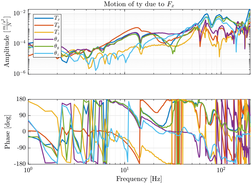
5.3 Analysis of some FRF
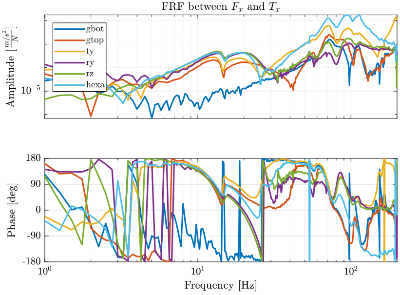
Figure 7: FRFs of all the 6 solid bodies in one direction
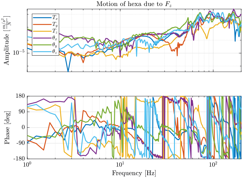
Figure 8: FRFs of one solid body in all its DOFs (expressed with a frame centered with its center of mass)
5.4 Save the FRF
save('mat/frf_com.mat', 'FRFs_CoM');