SpeedGoat

1. Setup
2. Signal Processing

1 Setup

Two L22 geophones are used. They are placed on the ID31 granite. They are leveled.

The signals are amplified using voltage amplifier with a gain of 60dB. The voltage amplifiers include a low pass filter with a cut-off frequency at 1kHz.

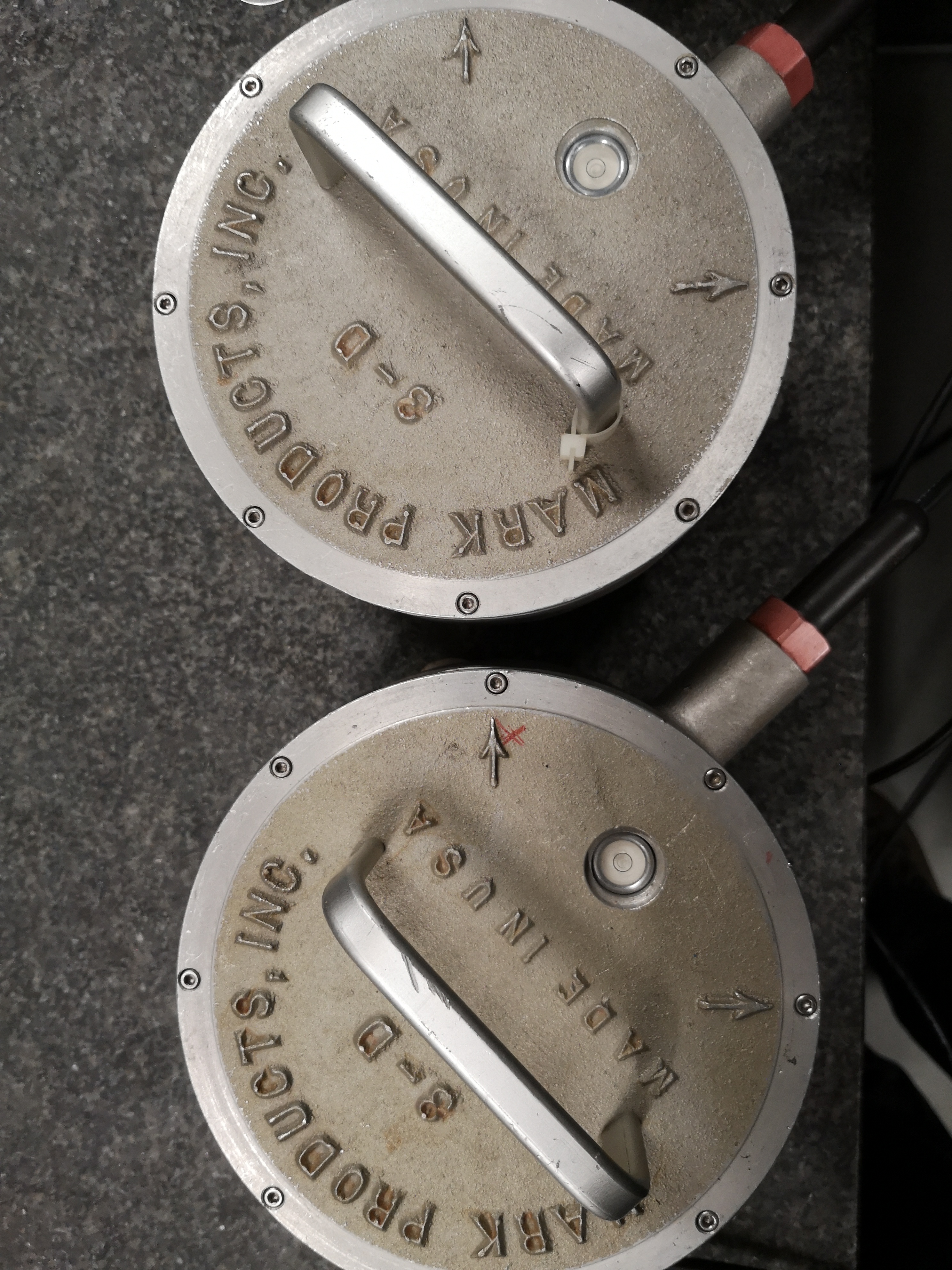
Figure 1: Setup

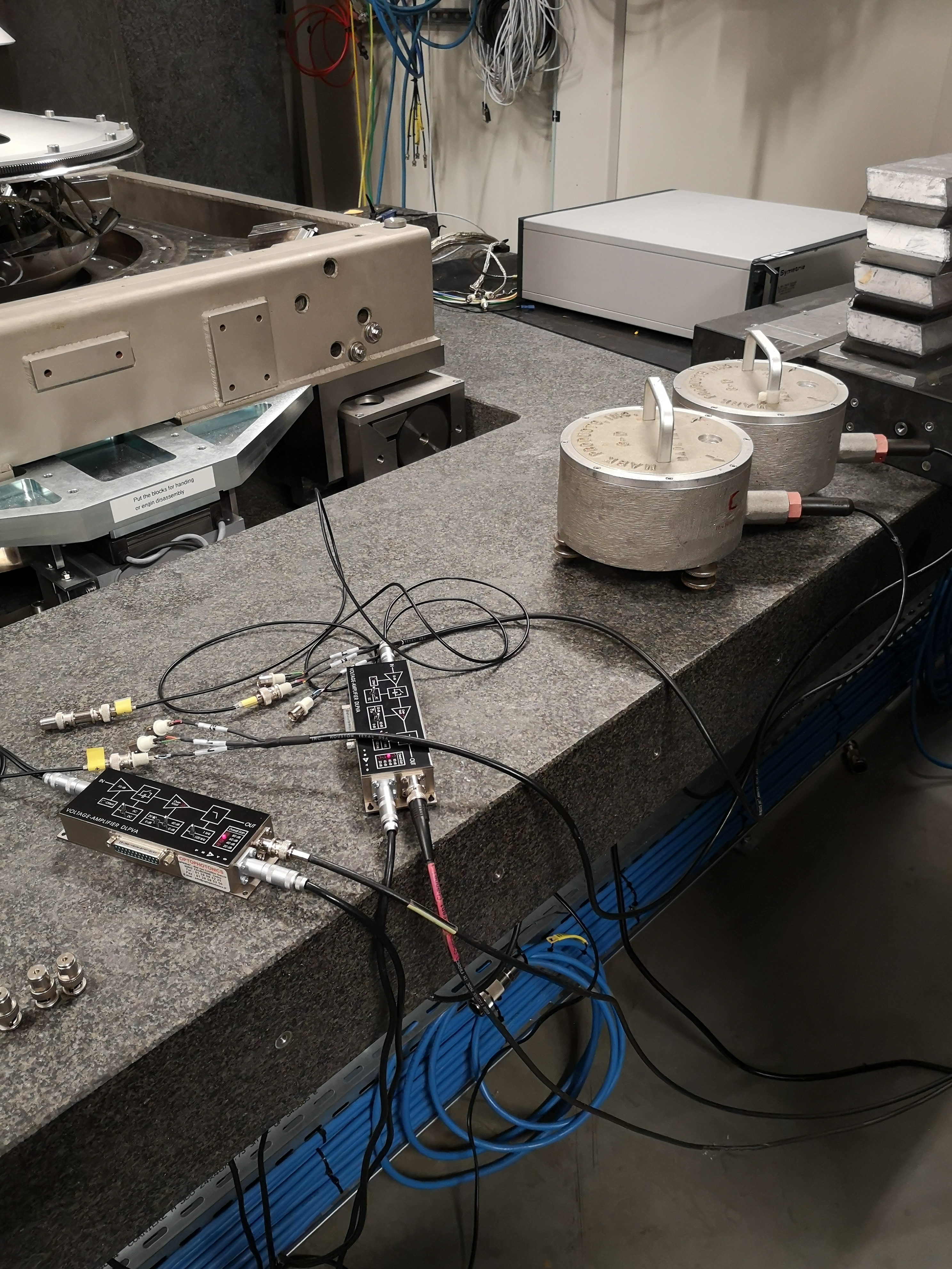
Figure 2: Geophones

2 Signal Processing

2.1 Load data

load('mat/data_001.mat', 't', 'x1', 'x2');
dt = t(2) - t(1);

2.2 Time Domain Data

figure;
hold on;
plot(t, x1);
plot(t, x2);
hold off;
xlabel('Time [s]');
ylabel('Voltage [V]');
xlim([t(1), t(end)]);

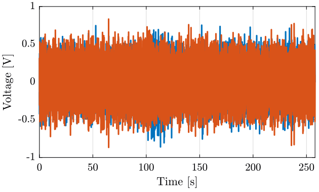
Figure 3: Time domain Data

figure;
hold on;
plot(t, x1);
plot(t, x2);
hold off;
xlabel('Time [s]');
ylabel('Voltage [V]');
xlim([0 1]);

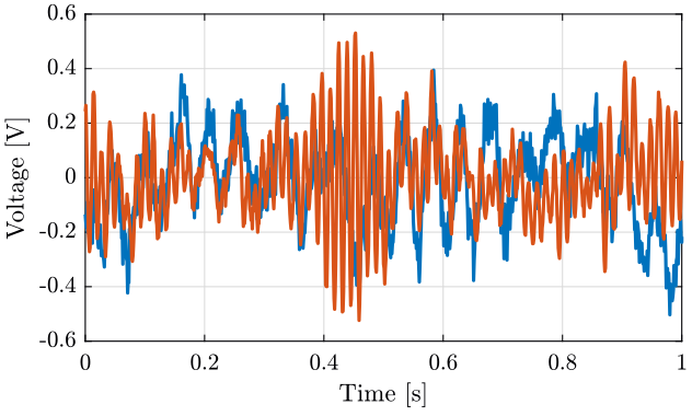
Figure 4: Time domain Data - Zoom

2.3 Compute PSD

[pxx1, f1] = pwelch(x1, hanning(ceil(length(t)/100)), 0, [], 1/dt);
[pxx2, f2] = pwelch(x2, hanning(ceil(length(t)/100)), 0, [], 1/dt);

2.4 Take into account sensibility of Geophone

The Geophone used are L22.

S0 = 88; % Sensitivity [V/(m/s)]
f0 = 2; % Cut-off frequnecy [Hz]
S = (s/2/pi/f0)/(1+s/2/pi/f0);

figure;
bodeFig({S});
ylabel('Amplitude [V/(m/s)]')

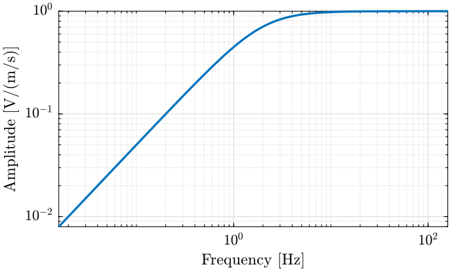
Figure 5: Sensibility of the Geophone

We take into account the gain of the electronics. The cut-off frequency is set at 1kHz.

[ ] Check what is the order of the filter
[ ] Maybe I should not use this filter as there is no high frequencies anyway?

G0 = 60; % [dB]

G = G0/(1+s/2/pi/1000);

figure;
hold on;
plot(f1, sqrt(pxx1)./squeeze(abs(freqresp(G, f1, 'Hz')))./squeeze(abs(freqresp(S, f1, 'Hz'))));
plot(f2, sqrt(pxx2)./squeeze(abs(freqresp(G, f2, 'Hz')))./squeeze(abs(freqresp(S, f2, 'Hz'))));
hold off;
set(gca, 'xscale', 'log');
set(gca, 'yscale', 'log');
xlabel('Frequency [Hz]'); ylabel('PSD [m/s/sqrt(Hz)]')

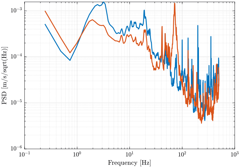
Figure 6: Spectral density of the velocity