Modal Analysis
Table of Contents
1 Goal
The goal is to experimentally extract a Spatial Model (mass, damping, stiffness) of the structure (shown on figure 1) in order to tune the Multi-Body model.
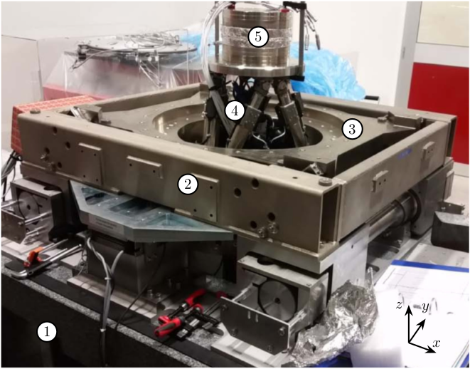
Figure 1: Picture of the ID31 Micro-Station. (1) Granite (2) Translation Stage (3) Tilt Stage (4) Hexapod (5) Dummy Mass
The procedure is represented on figure 2 where we go from left to right.

Figure 2: Vibration Analysis Procedure
First, we obtain a Response Model (Frequency Response Functions) from measurements. This is further converted into a Modal Model (Natural Frequencies and Mode Shapes). Finally, this is converted into a Spatial Model with the Mass/Damping/Stiffness matrices.
Theses matrices will be used to tune the Simscape (multi-body) model.
The modes we want to identify are those in the frequency range between 0Hz and 150Hz.
2 Type of Model
The model that we want to obtain is a multi-body model. It is composed of several solid bodies connected with springs and dampers. The solid bodies are represented with different colors on figure 3.
In the simscape model, the solid bodies are:
- the granite (1 or 2 solids)
- the translation stage
- the tilt stage
- the spindle and slip-ring
- the hexapod
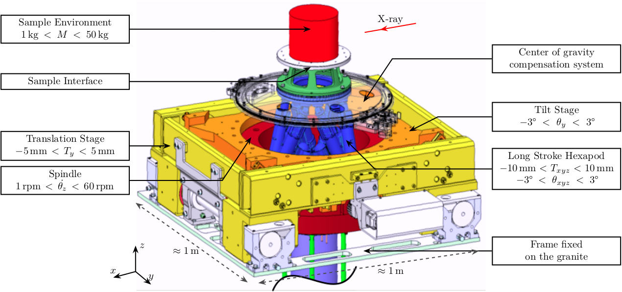
Figure 3: CAD view of the ID31 Micro-Station
However, each of the DOF of the system may not be relevant for the modes present in the frequency band of interest. For instance, the translation stage may not vibrate in the Z direction for all the modes identified. Then, we can block this DOF and this simplifies the model.
The modal identification done here will thus permit us to determine which DOF can be neglected.
3 Instrumentation Used
In order to perform to Modal Analysis and to obtain first a Response Model, the following devices are used:
- An acquisition system (OROS) with 24bits ADCs (figure 4)
- 3 tri-axis Accelerometers (figure 5) with parameters shown on table 1
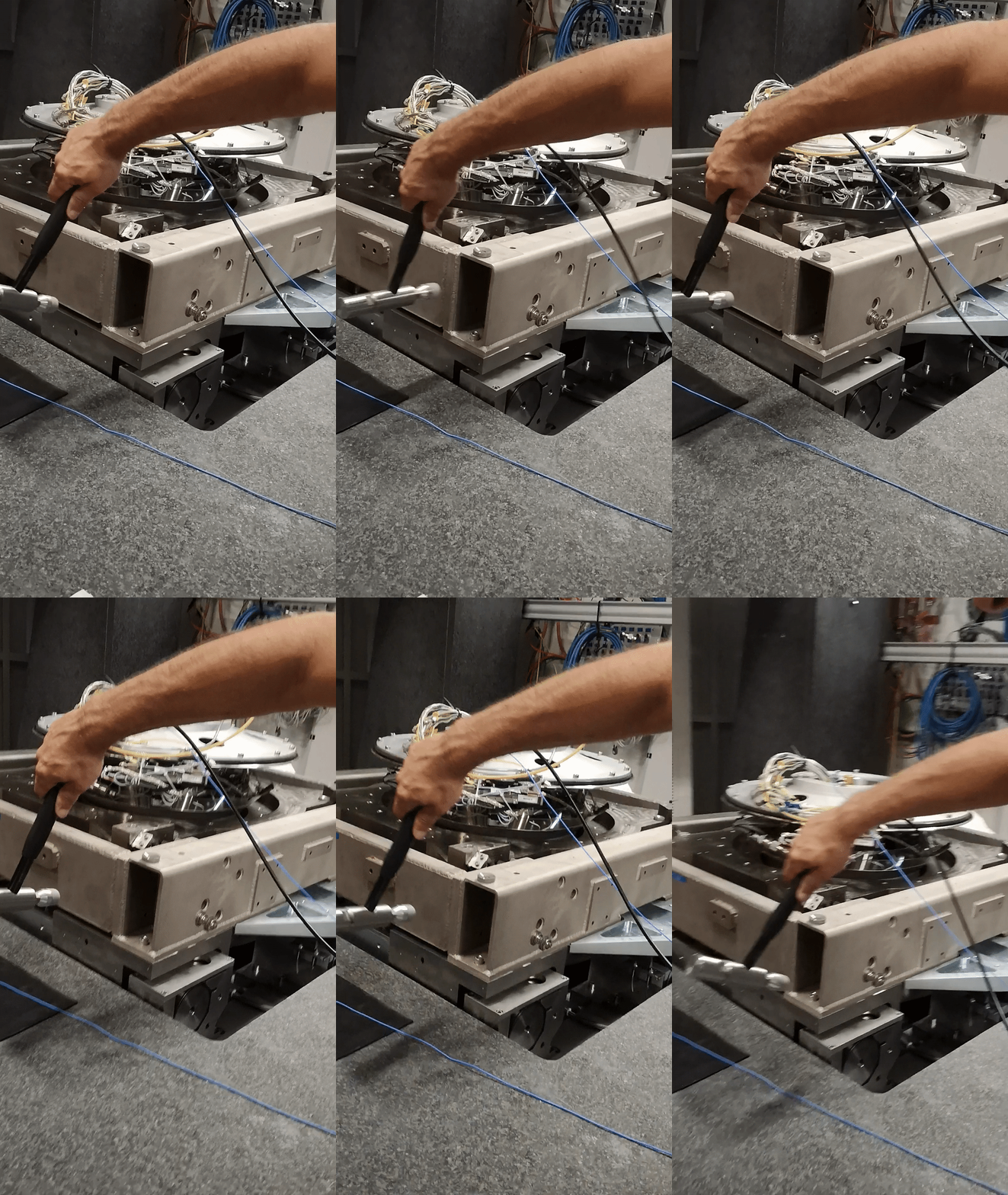
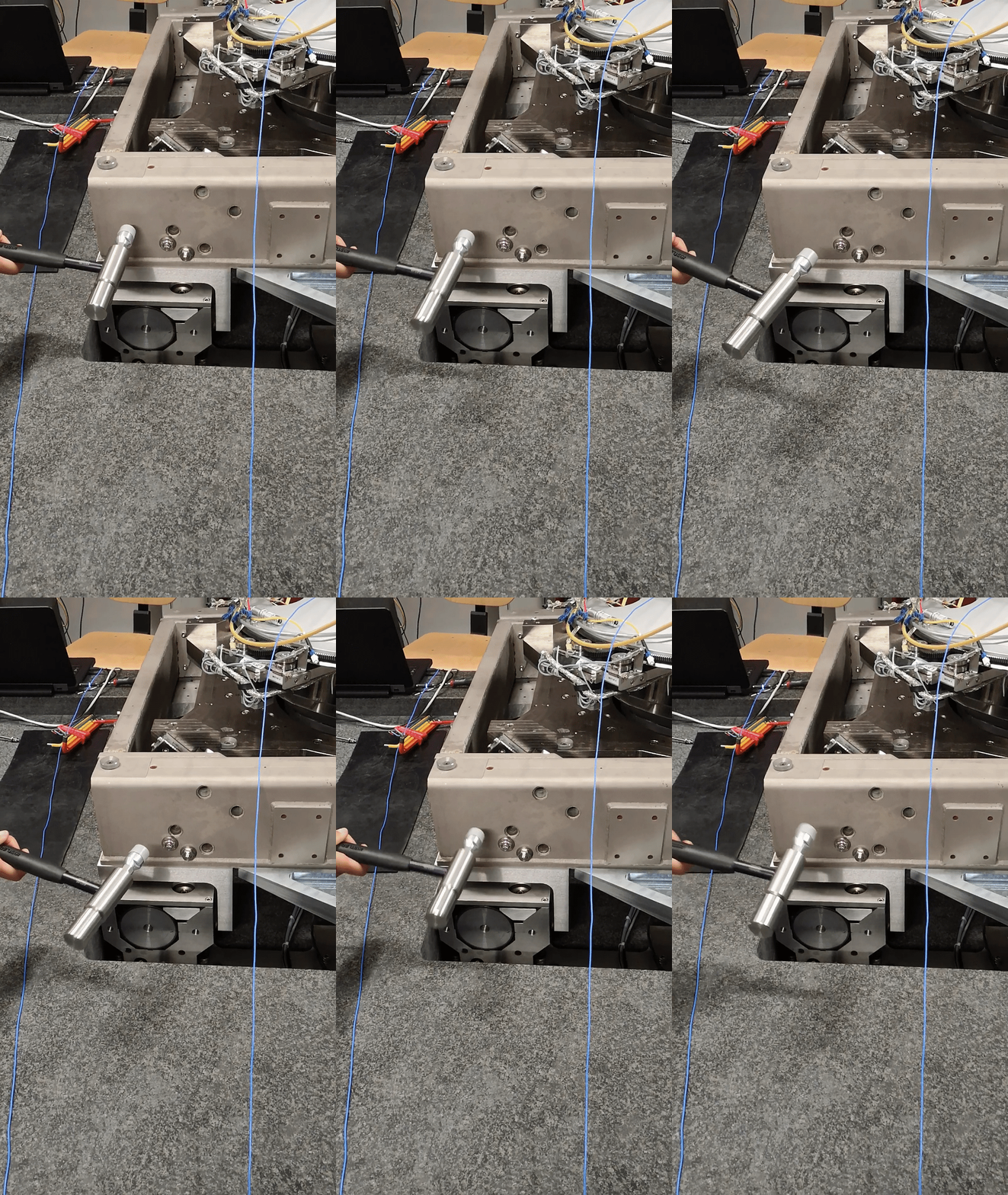
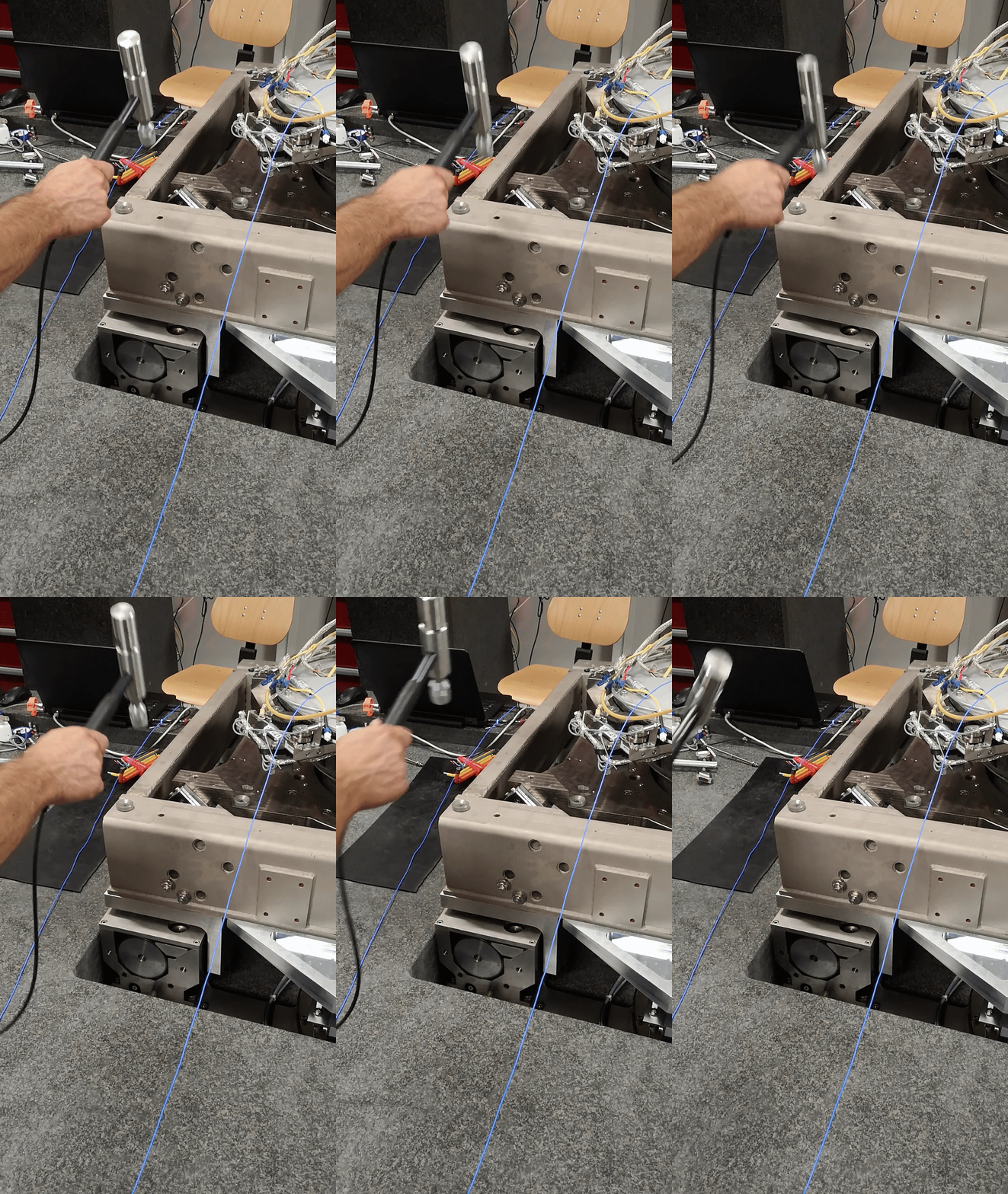
- An Instrumented Hammer with various Tips (figure 6) (figure 7)
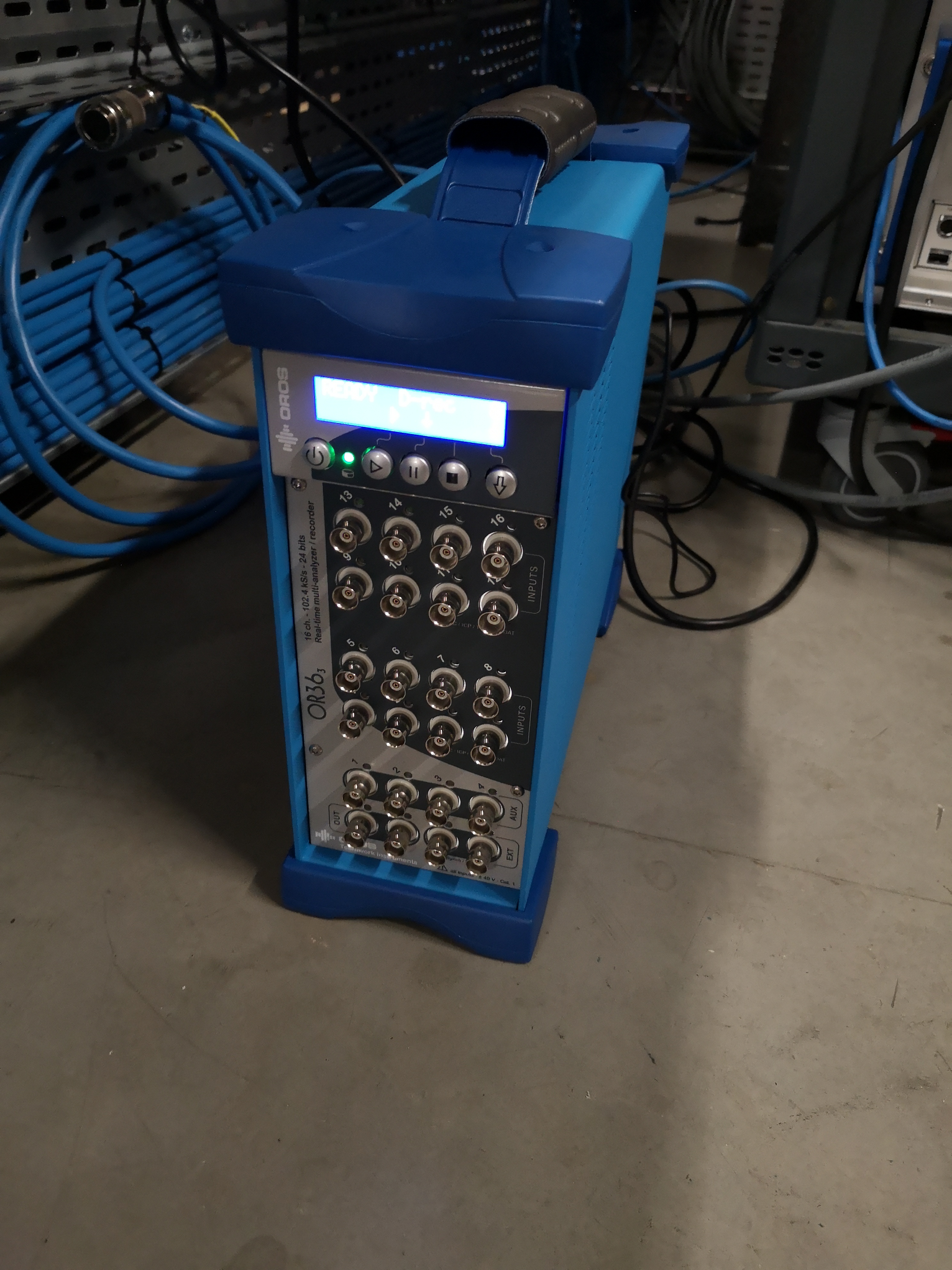
Figure 4: Acquisition system: OROS
The acquisition system permits to auto-range the inputs (probably using variable gain amplifiers) the obtain the maximum dynamic range. This is done before each measurement. Anti-aliasing filters are also included in the system.
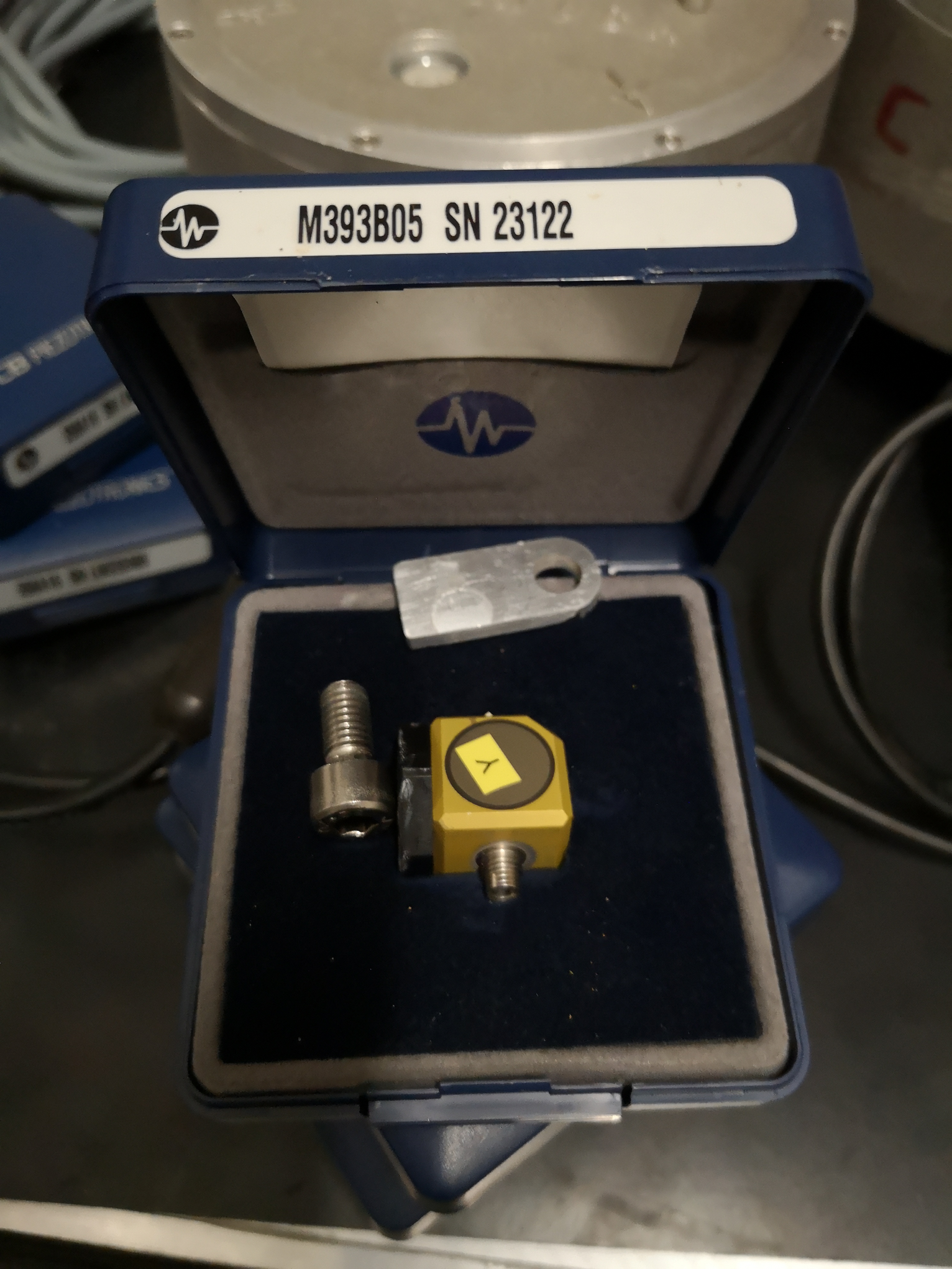
Figure 5: Accelerometer used: M393B05
| Sensitivity | 10V/g |
| Measurement Range | 0.5 g pk |
| Broadband Resolution | 0.000004 g rms |
| Frequency Range | 0.7 to 450Hz |
| Resonance Frequency | > 2.5kHz |
Tests have been conducted to determine the most suitable Hammer tip. This has been found that the softer tip gives the best results. It excites more the low frequency range where the coherence is low, the overall coherence was improved.
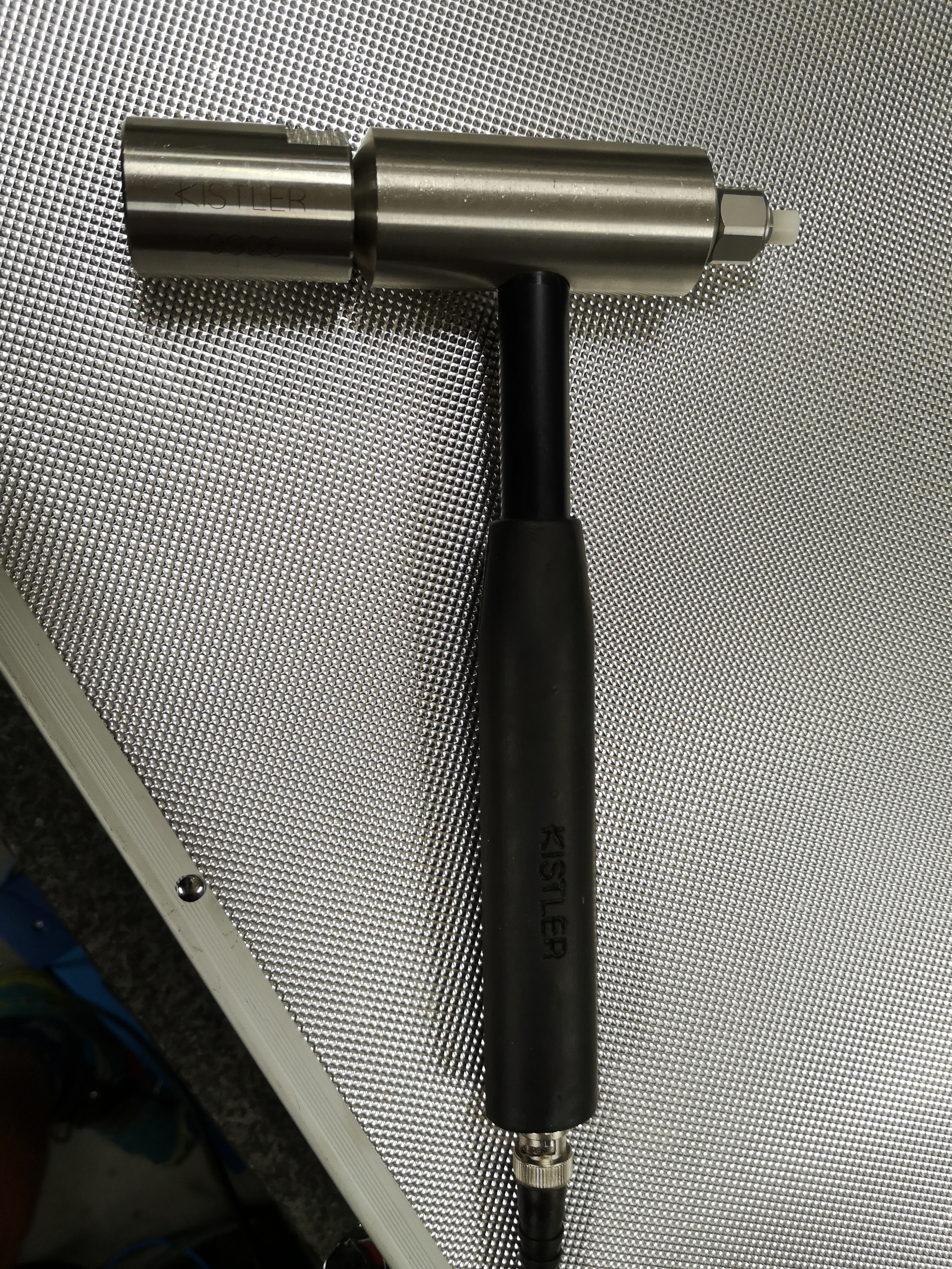
Figure 6: Instrumented Hammer
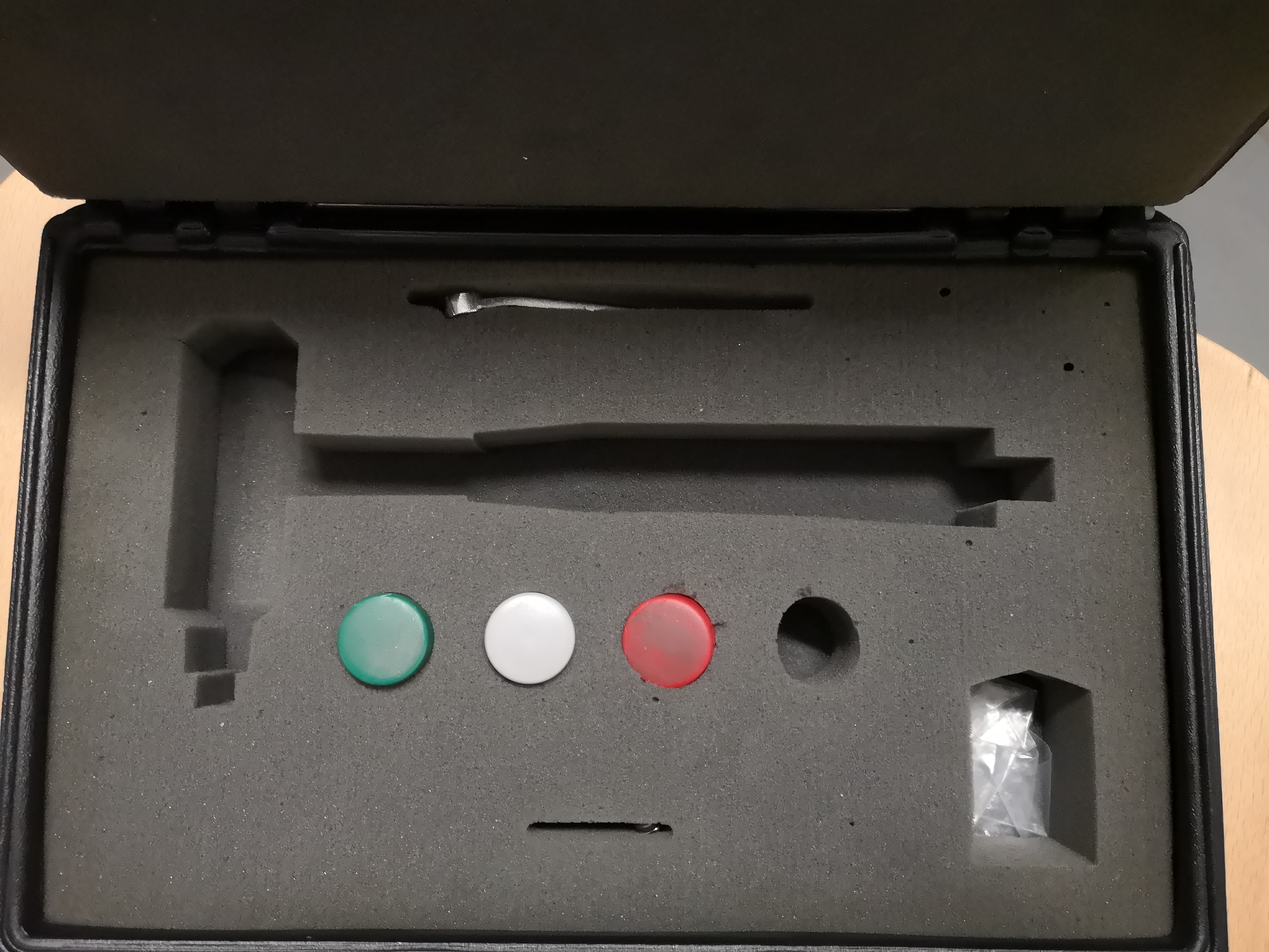
Figure 7: Hammer tips
The accelerometers are glued on the structure.
4 Structure Preparation and Test Planning
4.1 Structure Preparation
All the stages are turned ON. This is done for two reasons:
- Be closer to the real dynamic of the station in used
- If the control system of stages are turned OFF, this would results in very low frequency modes un-identifiable with the current setup, and this will also decouple the dynamics which would not be the case in practice
This is critical for the translation stage and the spindle as their is no stiffness in the free DOF (air-bearing for the spindle for instance).
The alternative would have been to mechanically block the stages with screws, but this may result in changing the modes.
The stages turned ON are:
- Translation Stage
- Tilt Stage
- Spindle and Slip-Ring
- Hexapod
The top part representing the NASS and the sample platform have been removed in order to reduce the complexity of the dynamics and also because this will be further added in the model inside Simscape.
All the stages are moved to their zero position (Ty, Ry, Rz, Slip-Ring, Hexapod).
All other elements have been remove from the granite such as another heavy positioning system.
4.2 Test Planing
The goal is to identify the full \(N \times N\) FRF matrix (where \(N\) is the number of degree of freedom of the system).
However, the principle of reciprocity states that: \[ H_{jk} = \frac{X_j}{F_k} = H_{kj} = \frac{X_k}{F_j} \] Thus, only one column or one line of the matrix has to be identified.
Either we choose to identify \(\frac{X_k}{F_i}\) or \(\frac{X_i}{F_k}\) for any chosen \(k\) and for \(i = 1,\ ...,\ N\).
We here choose to identify \(\frac{X_i}{F_k}\) for practical reasons:
- it is easier to glue the accelerometers on some stages than to excite this particular stage with the Hammer
The measurement thus consists of:
- always excite the structure at the same location with the Hammer
- Move the accelerometers to measure all the DOF of the structure
4.3 Location of the Accelerometers
4 tri-axis accelerometers are used for each solid body.
Only 2 could have been used as only 6DOF have to be measured, however, we have chosen to have some redundancy.
This could also help us identify measurement problems or flexible modes is present.
The position of the accelerometers are:
- 4 on the first granite
- 4 on the second granite (figure 8)
- 4 on top of the translation stage (figure 9)
- 4 on top of the tilt stage
- 4 on top of the spindle
- 4 on top of the hexapod (figure 10)
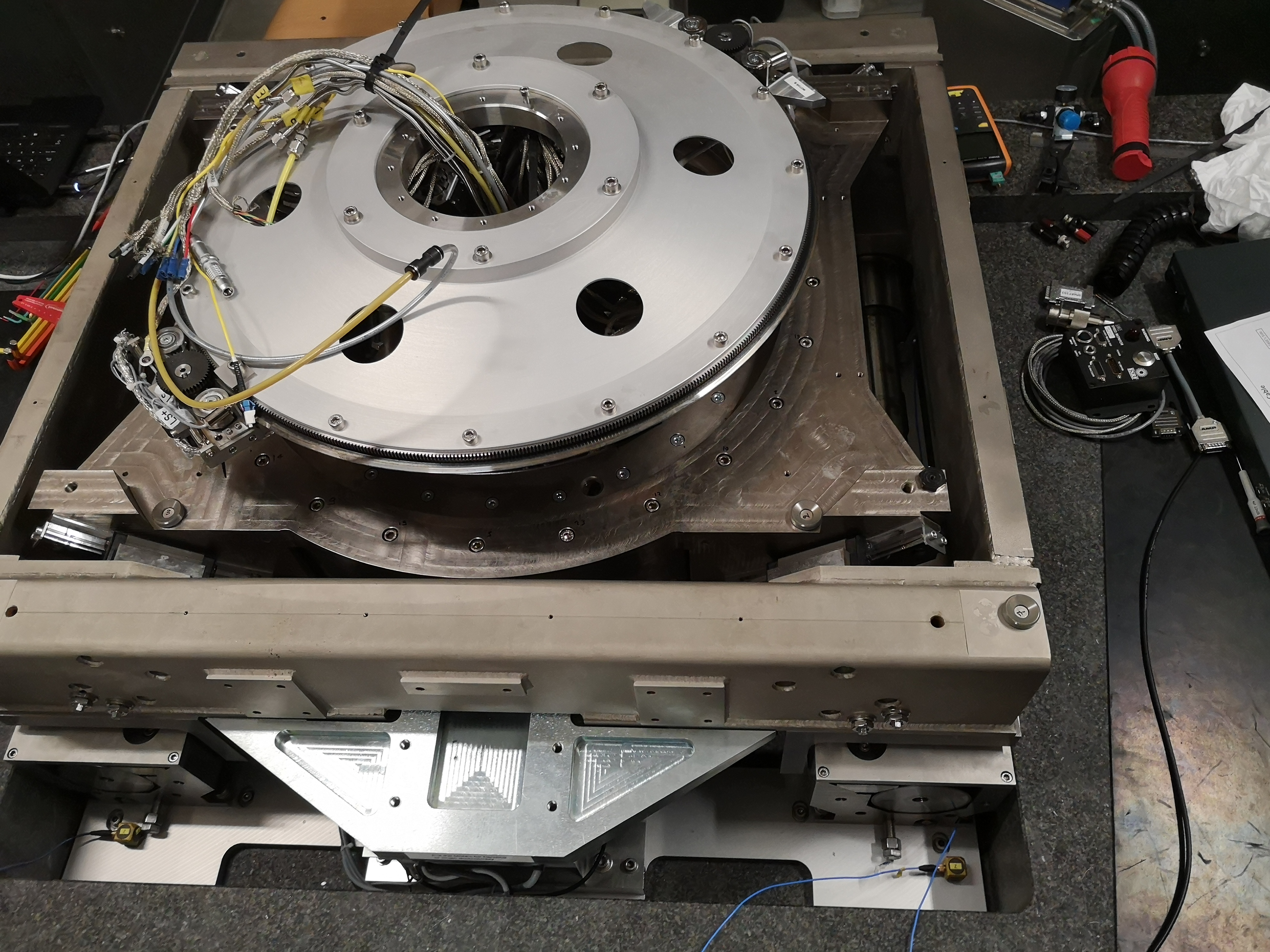
Figure 8: Accelerometers located on the top granite
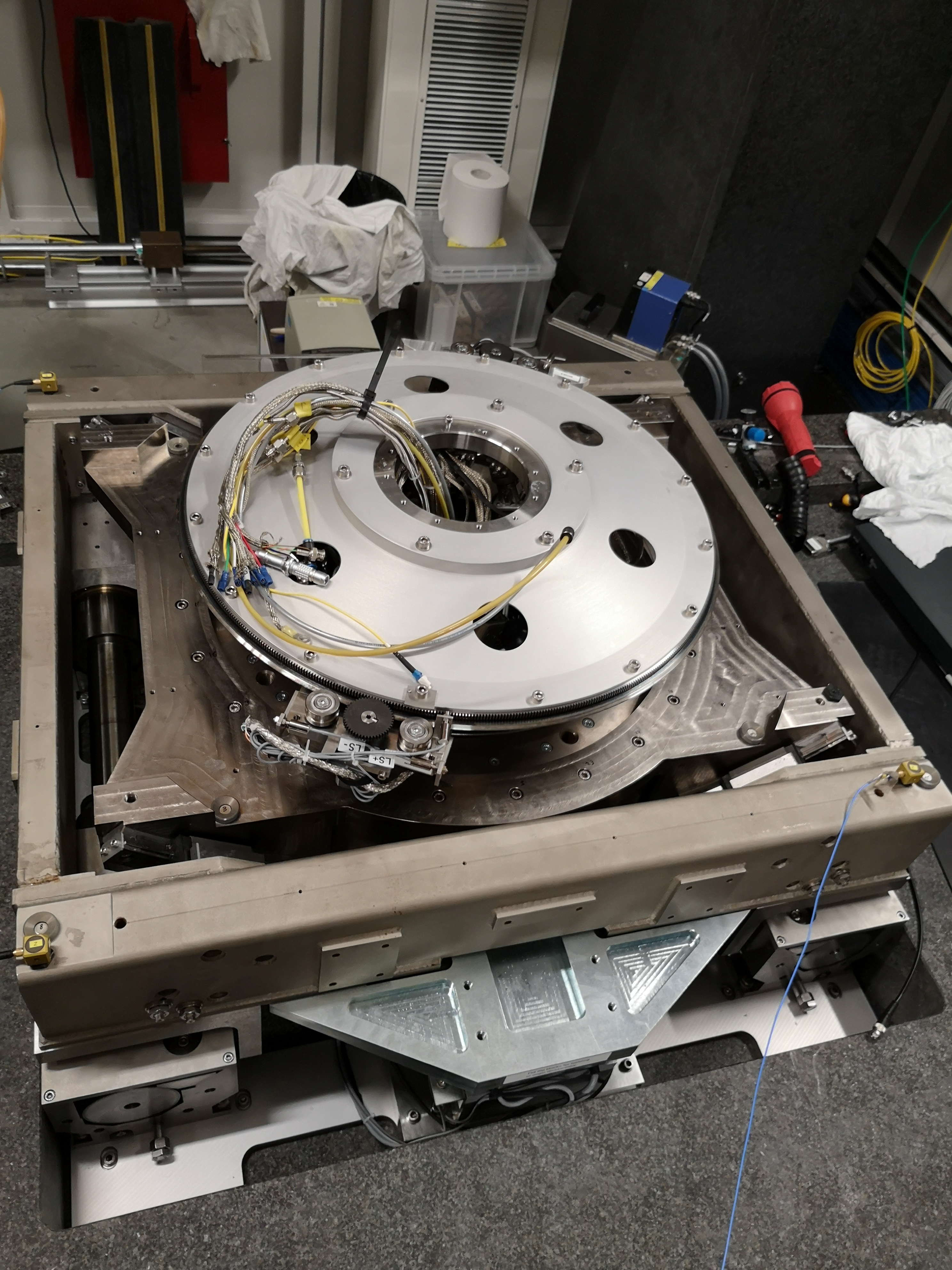
Figure 9: Accelerometers located on top of the translation stage
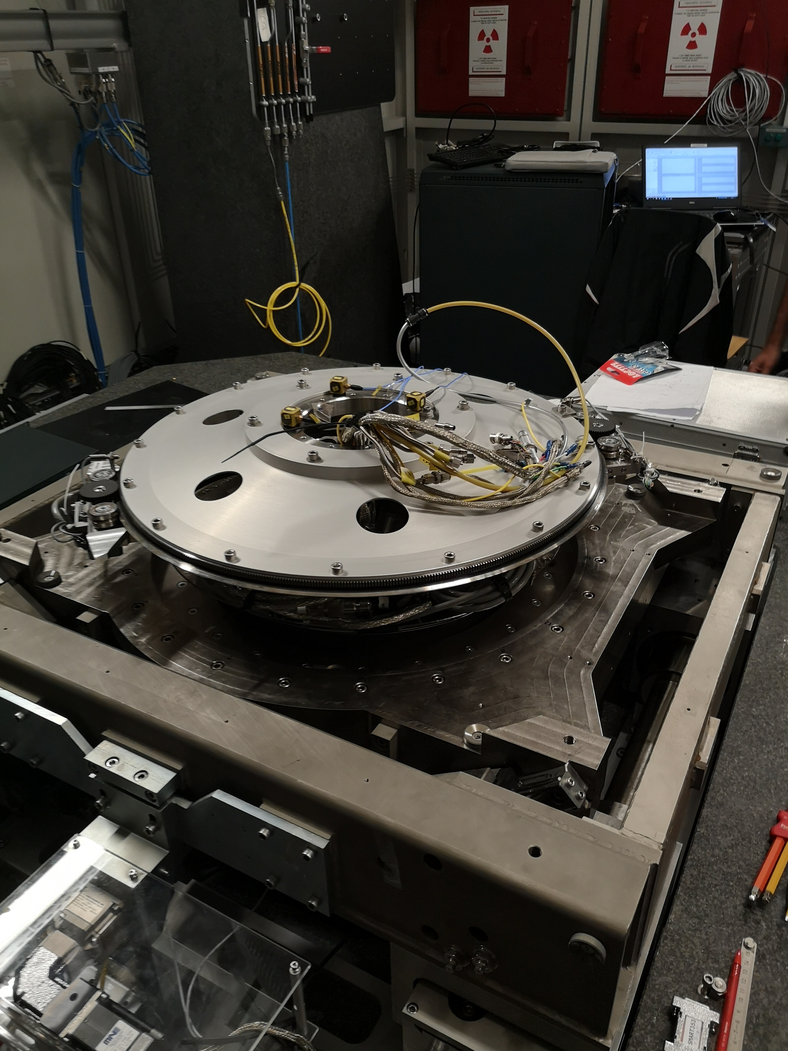
Figure 10: Accelerometers located on the Hexapod
5 Signal Processing
The measurements are averaged 10 times (figure 14) corresponding to 10 hammer impacts.
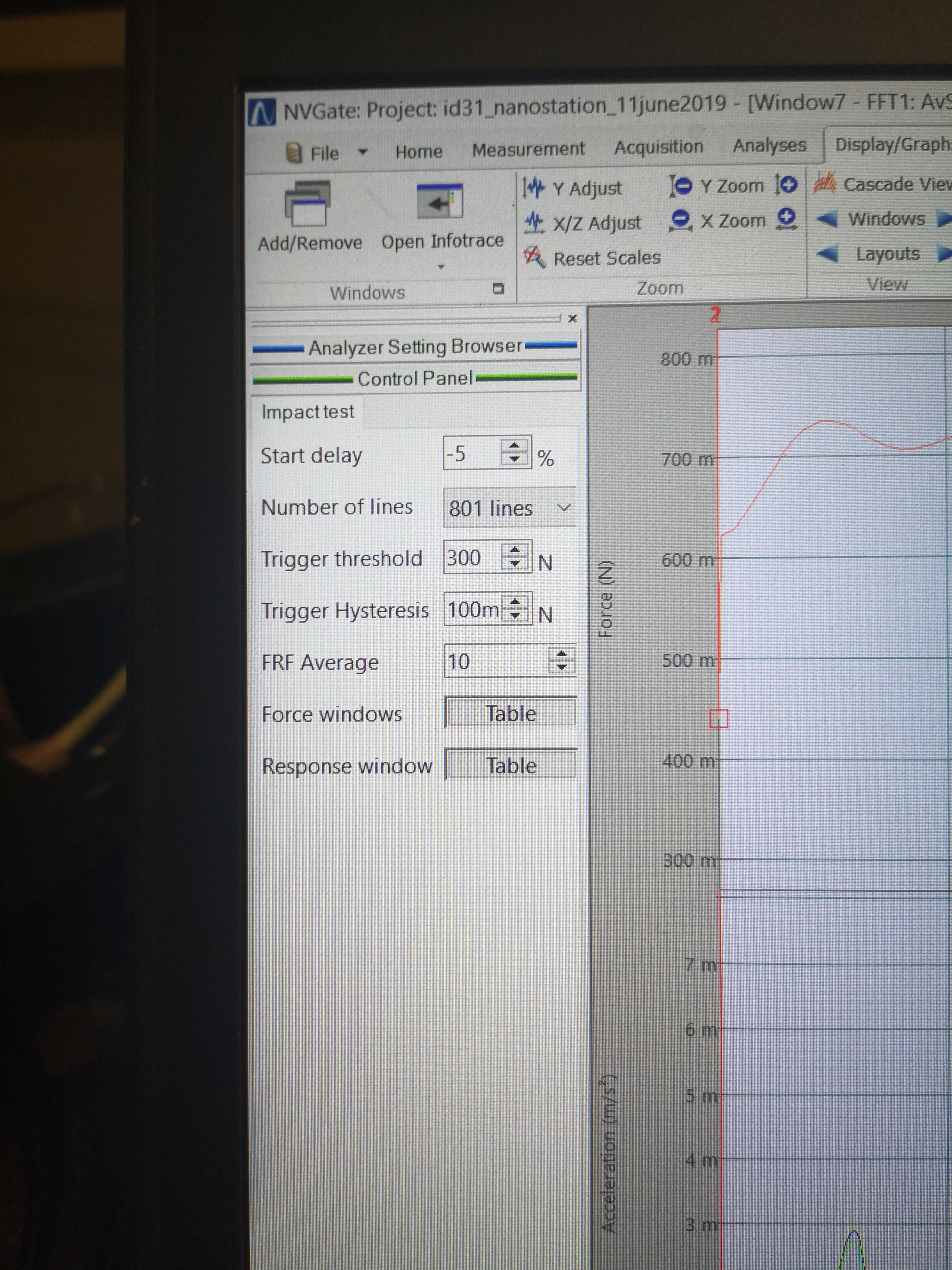
Figure 14: General Acquisition Settings
Windowing is used on the force response signals.
A boxcar window (figure 15) is used for the force signal as once the impact on the structure is done, the measured signal is meaningless.
An exponential window (figure 16) is used for the response signal as we are measuring transient signals and most of the information is located at the beginning of the signal.
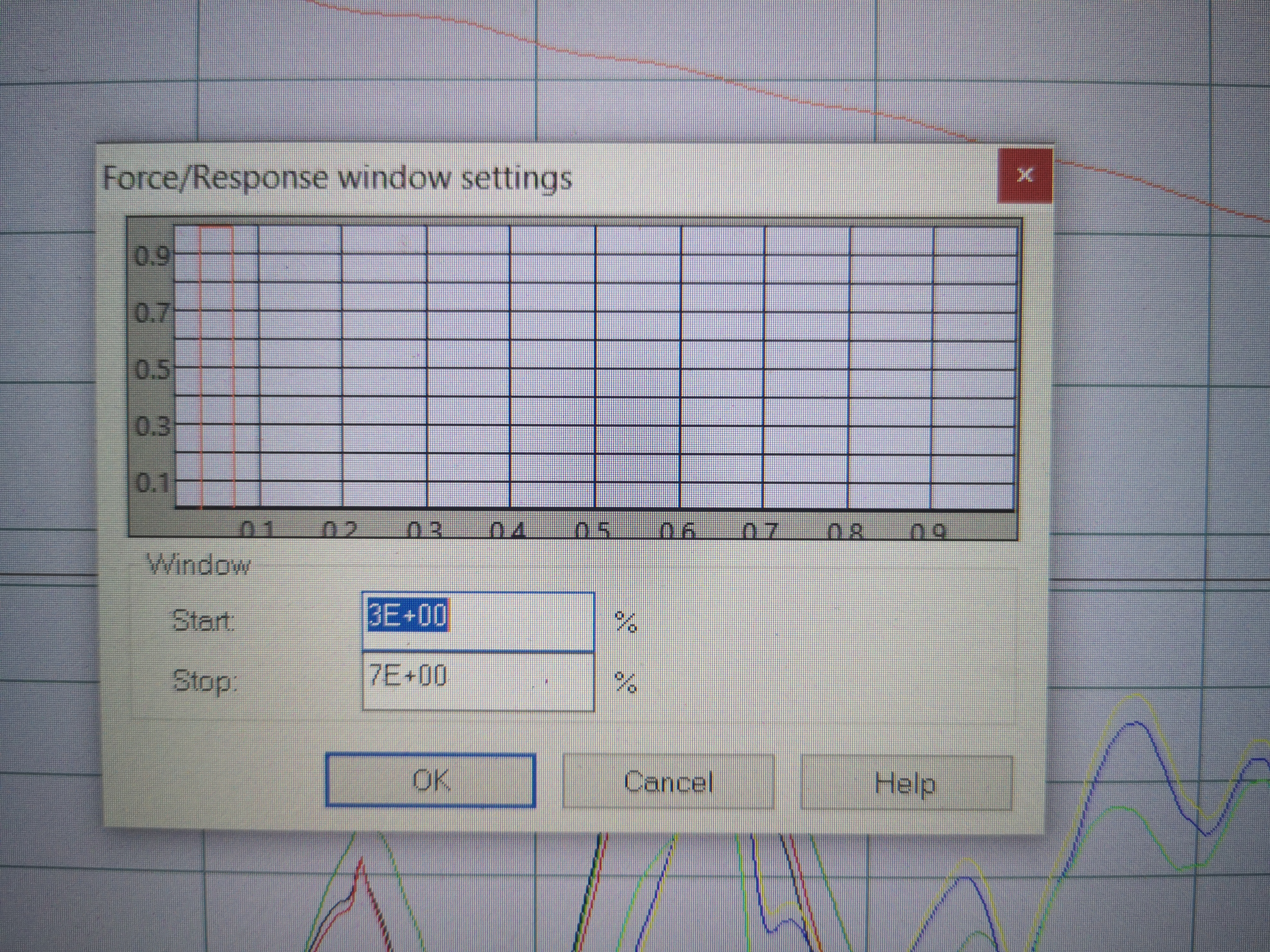
Figure 15: Window used for the force signal
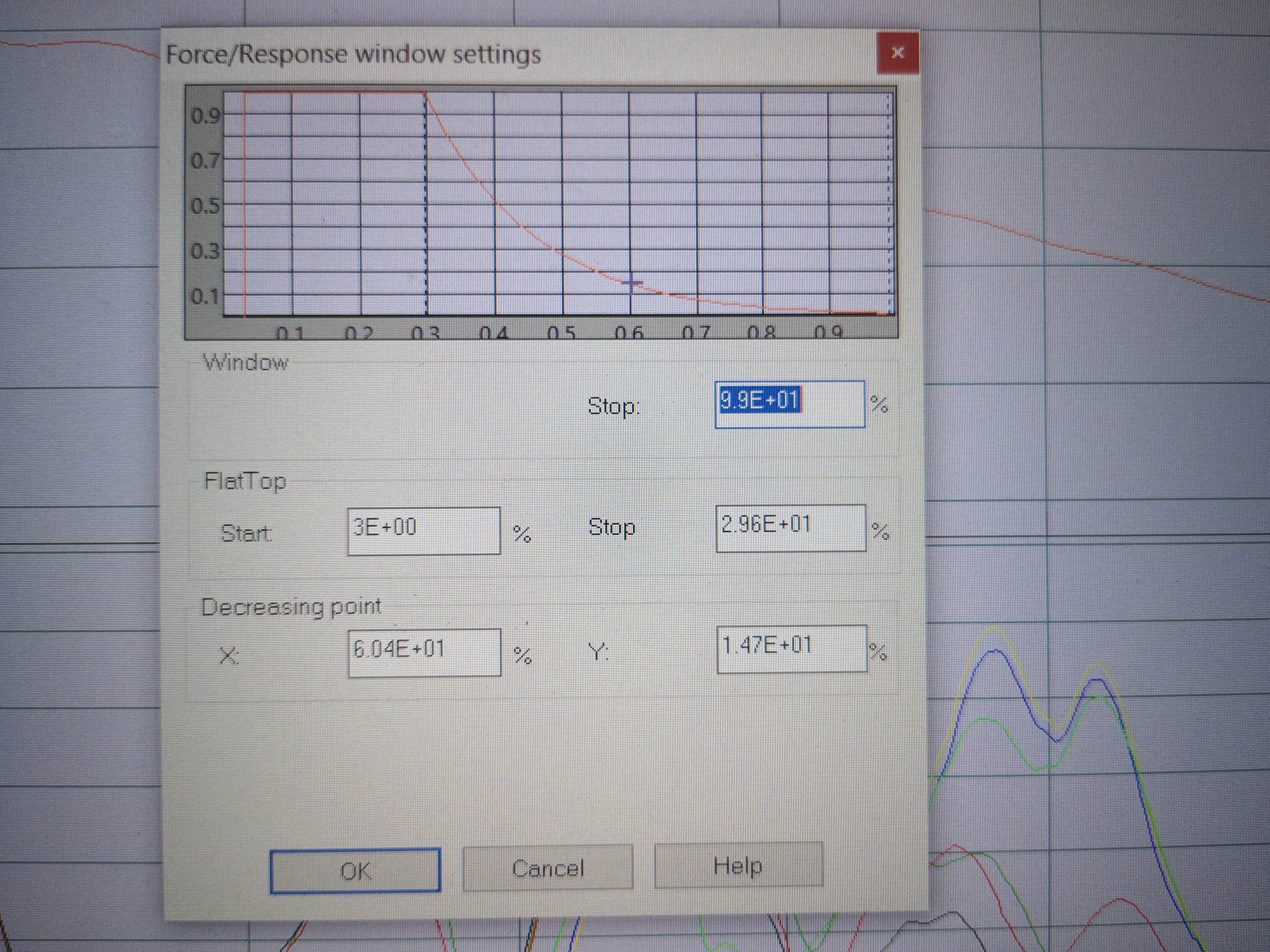
Figure 16: Window used for the response signal
6 Frequency Response Functions and Coherence Results
6.1 Load Data
meas1_raw = load('modal_analysis/raw_data/Measurement1.mat');
6.2 Raw Force Data
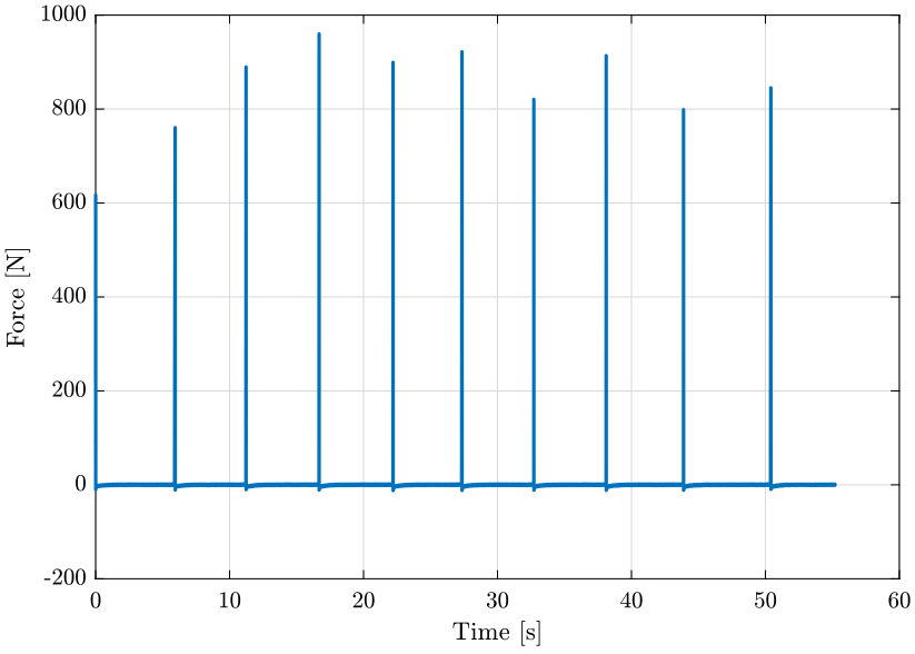
Figure 17: Raw Force Data from Hammer Blow
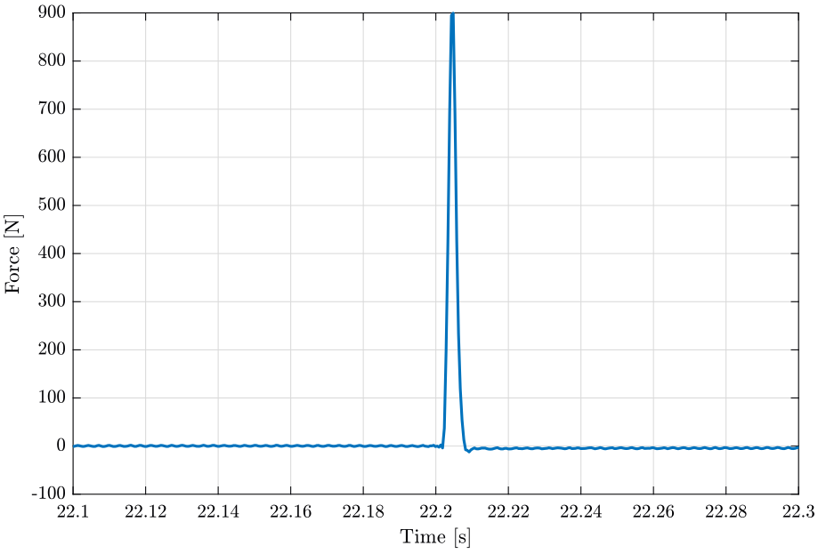
Figure 18: Raw Force Data from Hammer Blow - Zoom
6.3 Raw Response Data
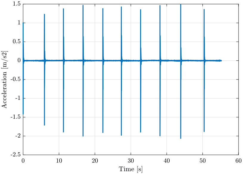
Figure 19: Raw Acceleration Data from Accelerometer
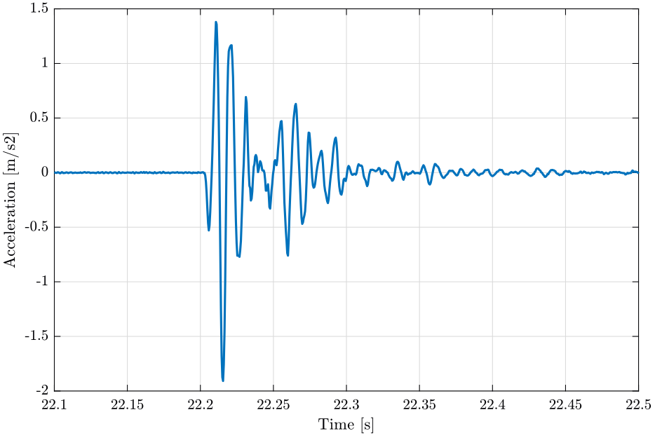
Figure 20: Raw Acceleration Data from Accelerometer - Zoom
6.4 Load Data
meas1 = load('modal_analysis/frf_coh/Measurement1.mat');
6.5 FRF and Coherence Results
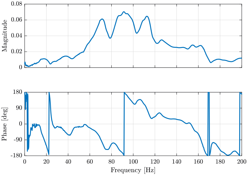
Figure 21: Example of one measured FRF
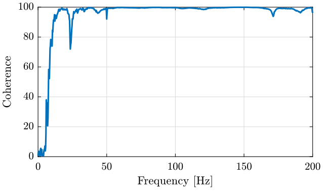
Figure 22: Example of one measured Coherence
7 Mode Shapes
Multiple modal extraction techniques can be used (SIMO, MIMO, narrow band, wide band, …). First preliminary results on 10 identified modes are presented here.
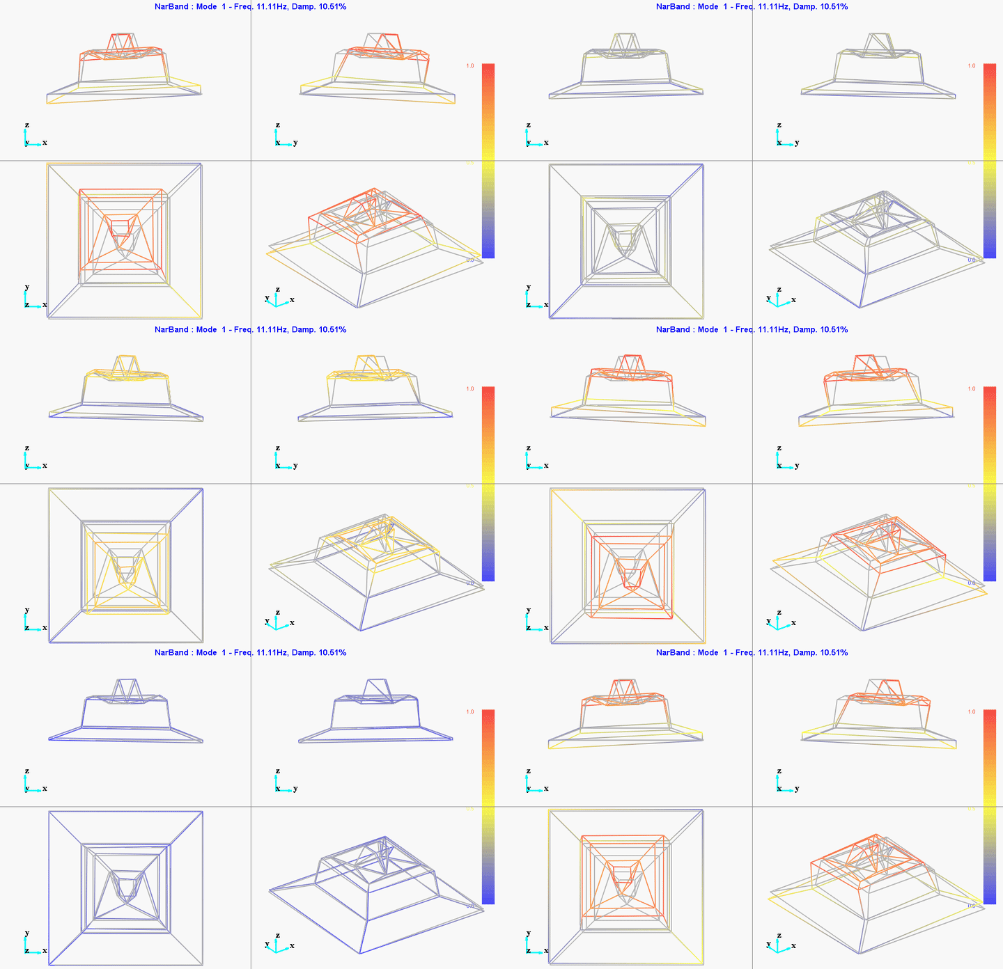
Figure 23: Mode 1
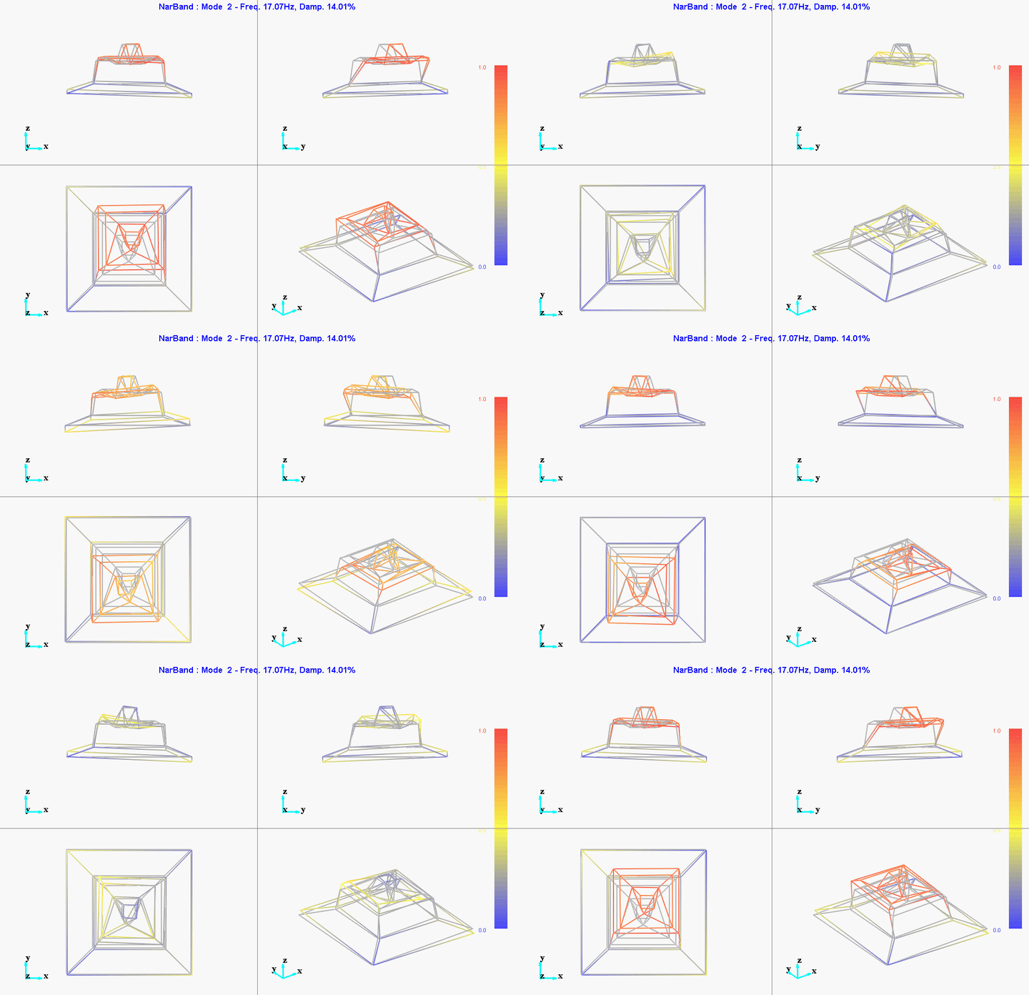
Figure 24: Mode 2
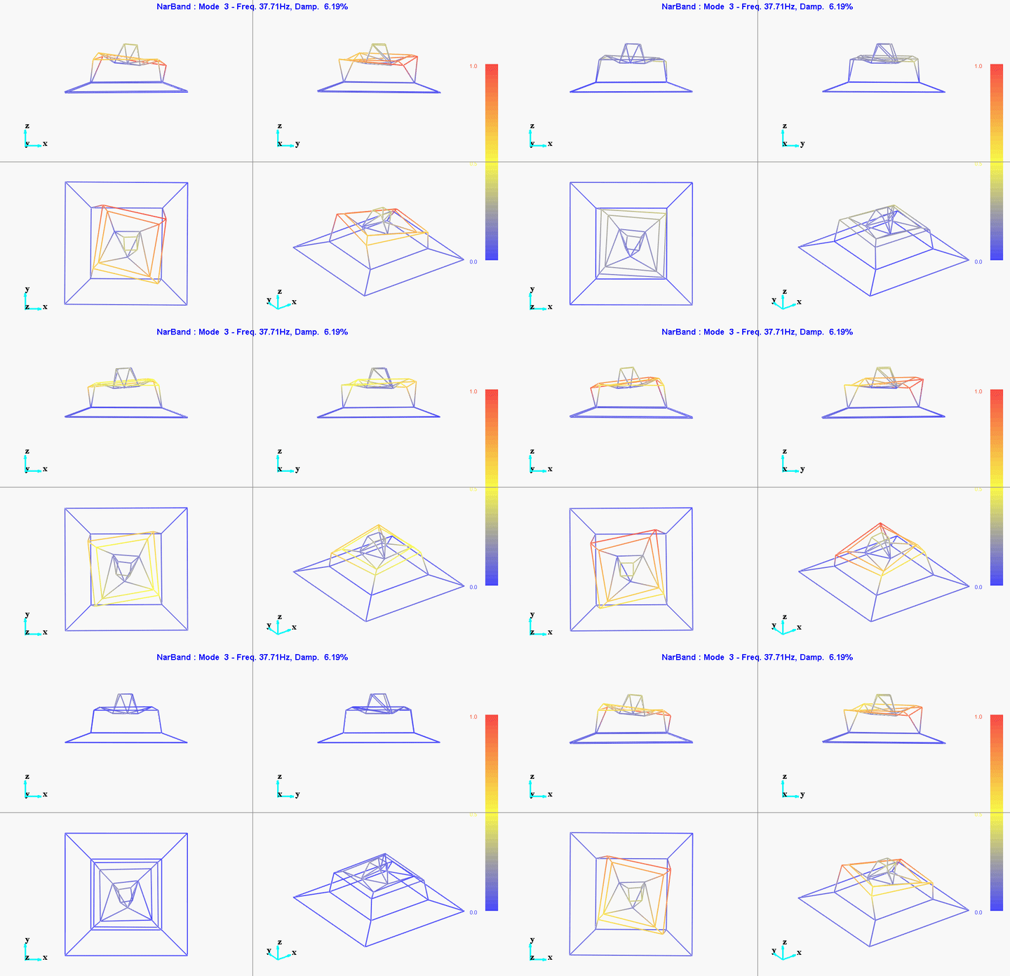
Figure 25: Mode 3
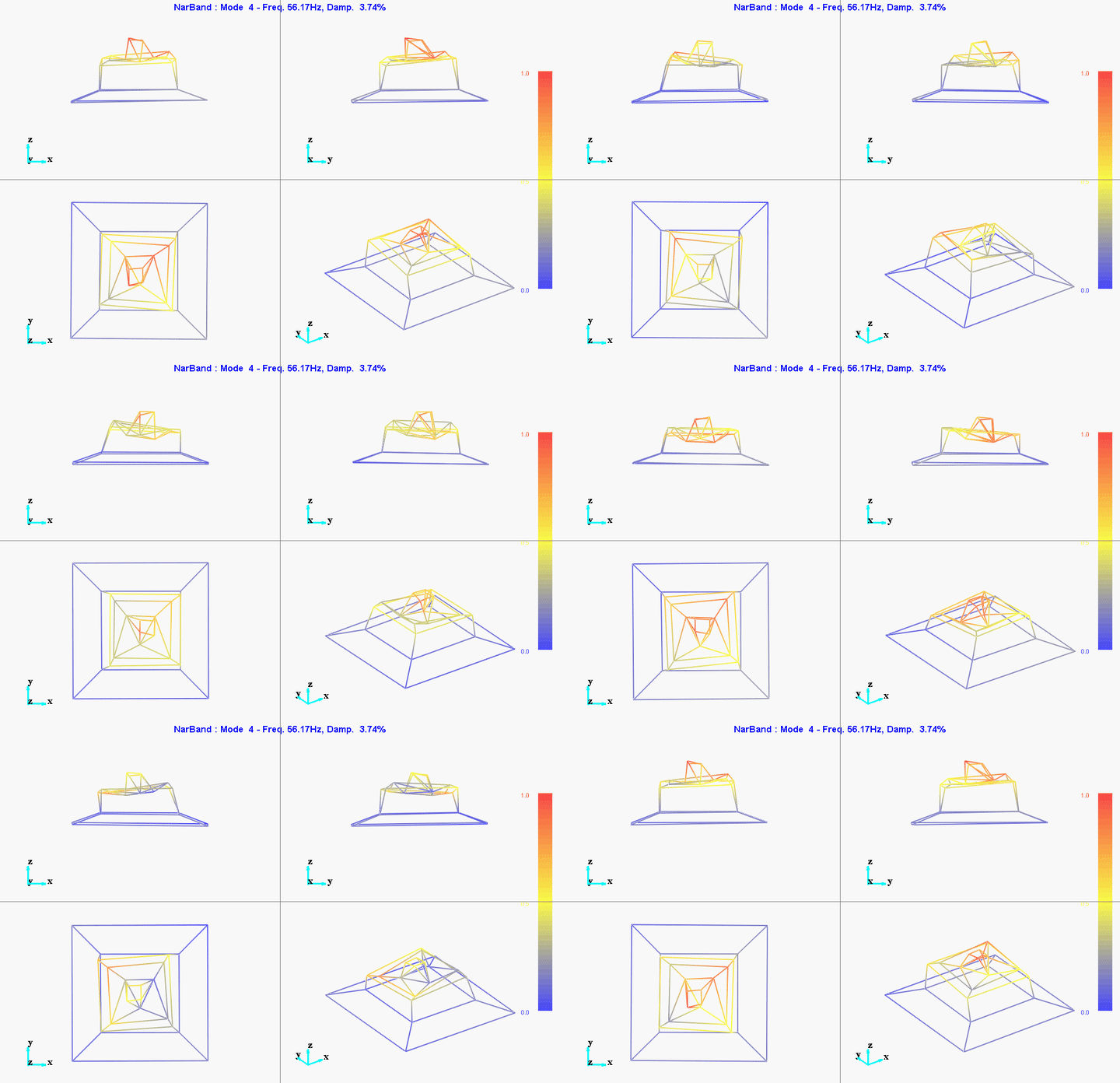
Figure 26: Mode 4
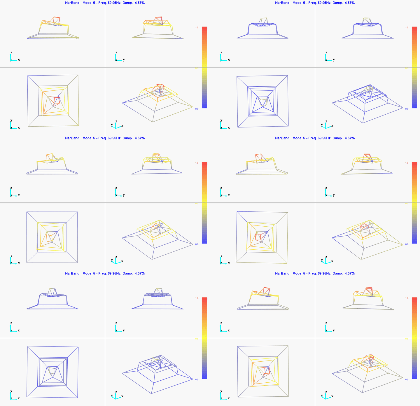
Figure 27: Mode 5
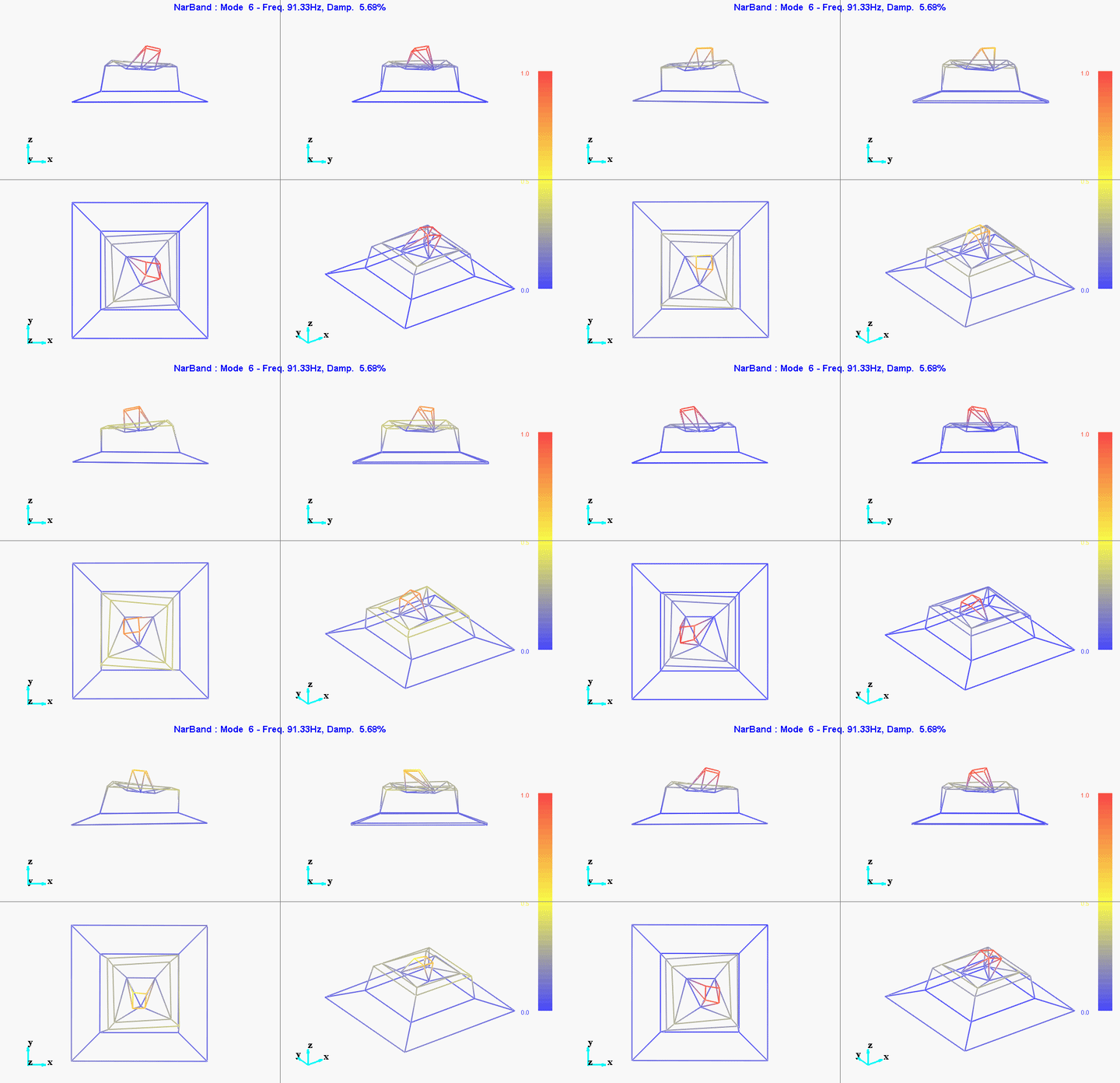
Figure 28: Mode 6
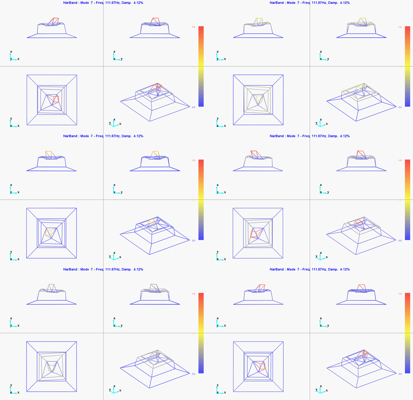
Figure 29: Mode 7

Figure 30: Mode 8
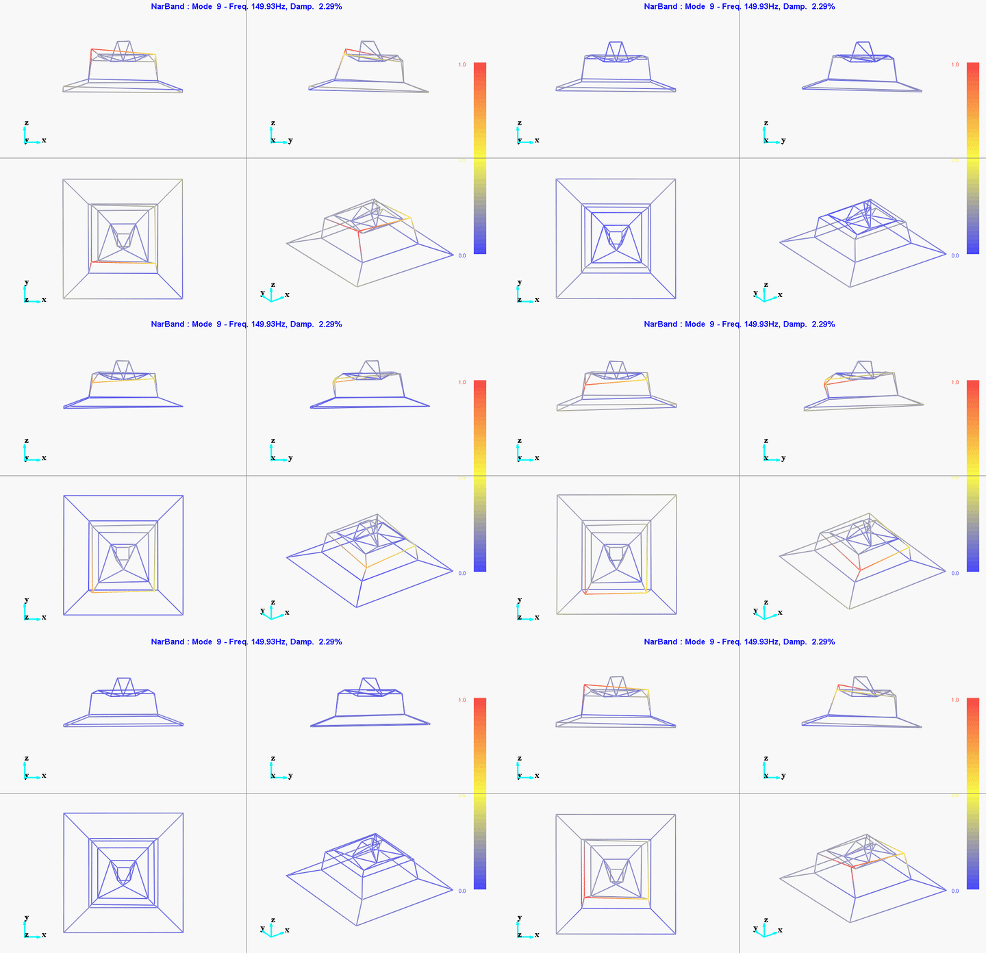
Figure 31: Mode 9
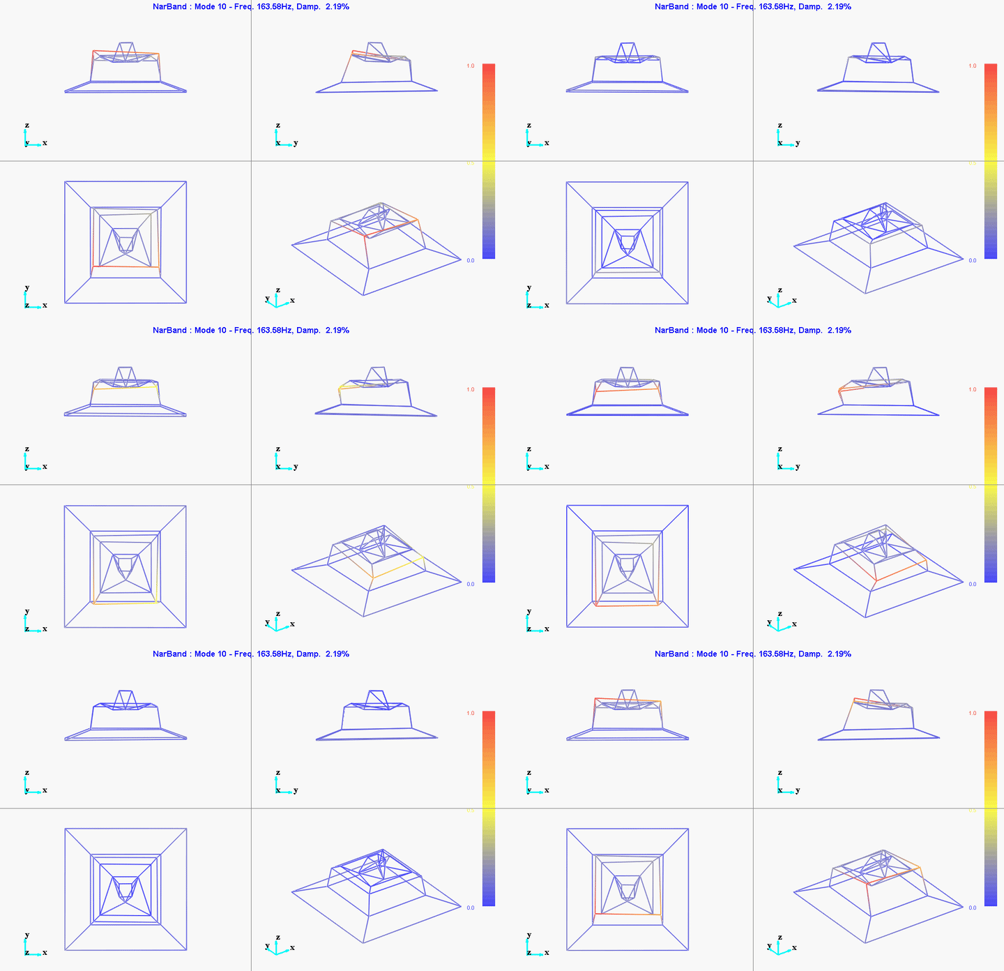
Figure 32: Mode 10
8 Obtained Modal Matrices
From the modal analysis software, we can export the obtained eigen matrices: \[ \begin{bmatrix} \omega_1^2 & & 0 \\ & \ddots & \\ 0 & & \omega_n^2 \end{bmatrix}; \quad \Psi = \begin{bmatrix} & & \\ \{\psi_1\} & \dots & \{\psi_n\} \\ & & \end{bmatrix} \]
where \(\bar{\omega}_r^2\) is the \(r^\text{th}\) eigenvalue squared and \(\{\phi\}_r\) is a description of the corresponding mode shape.
The file containing the eigen frequencies and mode shapes are shown below (for the first mode).
Created by N-Modal
Estimator: cmif
18-Jun-19 16:31:25


Mode 1
freq    = 11.11191Hz
damp    = 10.51401%
modal A =   8.52879e+003-2.29043e+003i
modal B =  -9.64203e+004-6.08978e+005i
Mode matrix of local coordinate [DOF: Re IM]
     1X+:  -9.34637e-002   4.52445e-002
     1Y+:   2.33790e-001   1.41439e-003
     1Z+:  -1.73754e-002   6.02449e-003
     2X+:  -7.42108e-002   3.91543e-002
     2Y+:   2.41566e-001  -1.44869e-003
     2Z+:  -5.99285e-003   2.10370e-003
     4X+:  -1.02163e-001   2.79561e-002
     4Y+:   2.29048e-001   2.89782e-002
     4Z+:  -2.85130e-002   1.77132e-004
     5X+:  -8.77132e-002   3.34081e-002
     5Y+:   2.14182e-001   2.14655e-002
     5Z+:  -1.54521e-002   1.26682e-002
     6X+:  -7.90143e-002   2.42583e-002
     6Y+:   2.20669e-001   2.12738e-002
     6Z+:   4.60755e-002   4.96406e-003
     7X+:  -7.79654e-002   2.58385e-002
     7Y+:   2.06861e-001   3.48019e-002
     7Z+:  -1.78311e-002  -1.29704e-002
     8X+:  -8.49357e-002   3.55200e-002
     8Y+:   2.07470e-001   3.59745e-002
     8Z+:  -7.66974e-002  -3.19813e-003
     9X+:  -7.38565e-002   1.95146e-002
     9Y+:   2.17403e-001   2.01550e-002
     9Z+:  -1.77073e-002  -3.46414e-003
    10X+:  -7.77587e-002   2.36700e-002
    10Y+:   2.35654e-001  -2.14540e-002
    10Z+:   7.94165e-002  -2.45897e-002
    11X+:  -8.17972e-002   2.20583e-002
    11Y+:   2.20906e-001  -4.30164e-003
    11Z+:  -5.60520e-003   3.10187e-003
    12X+:  -8.64261e-002   3.66022e-002
    12Y+:   2.15000e-001  -5.74661e-003
    12Z+:  -1.22622e-001   4.11767e-002
    13X+:  -4.25169e-002   1.56602e-002
    13Y+:   5.31036e-002  -1.73951e-002
    13Z+:  -4.07130e-002   1.26884e-002
    14X+:  -3.85032e-002   1.29431e-002
    14Y+:   5.36716e-002  -1.80868e-002
    14Z+:   1.00367e-001  -3.48798e-002
    15X+:  -4.25524e-002   1.46363e-002
    15Y+:   5.19668e-002  -1.69744e-002
    15Z+:   5.89747e-003  -2.32428e-003
    16X+:  -4.31268e-002   1.38332e-002
    16Y+:   5.07545e-002  -1.53045e-002
    16Z+:  -1.04172e-001   3.17984e-002
    17X+:  -2.69757e-002   9.07955e-003
    17Y+:   3.07837e-002  -9.44663e-003
    17Z+:  -7.63502e-003   1.68203e-003
    18X+:  -3.00097e-002   9.23966e-003
    18Y+:   2.83585e-002  -8.97747e-003
    18Z+:   1.52467e-001  -4.78675e-002
    19X+:  -2.70223e-002   6.16478e-003
    19Y+:   3.06149e-002  -6.25382e-003
    19Z+:  -4.84888e-003   1.93970e-003
    20X+:  -2.90976e-002   7.13184e-003
    20Y+:   3.36738e-002  -7.30875e-003
    20Z+:  -1.66902e-001   3.93419e-002
     3X+:  -9.40720e-002   3.93724e-002
     3Y+:   2.52307e-001   0.00000e+000
     3Z+:  -1.53864e-002  -9.25720e-004
    21X+:  -7.91940e-002   4.39648e-002
    21Y+:   2.04567e-001   9.49987e-003
    21Z+:  -1.56087e-002   7.08838e-003
    22X+:  -1.01070e-001   3.13534e-002
    22Y+:   1.92270e-001   1.80423e-002
    22Z+:   2.93053e-003  -1.97308e-003
    23X+:  -8.86455e-002   4.29906e-002
    23Z+:  -3.38351e-002   1.81362e-003
    23Y-:  -1.90862e-001  -2.53414e-002
9 Problem with AirLoc System
4 Airloc Levelers are used for the granite (figure 33).
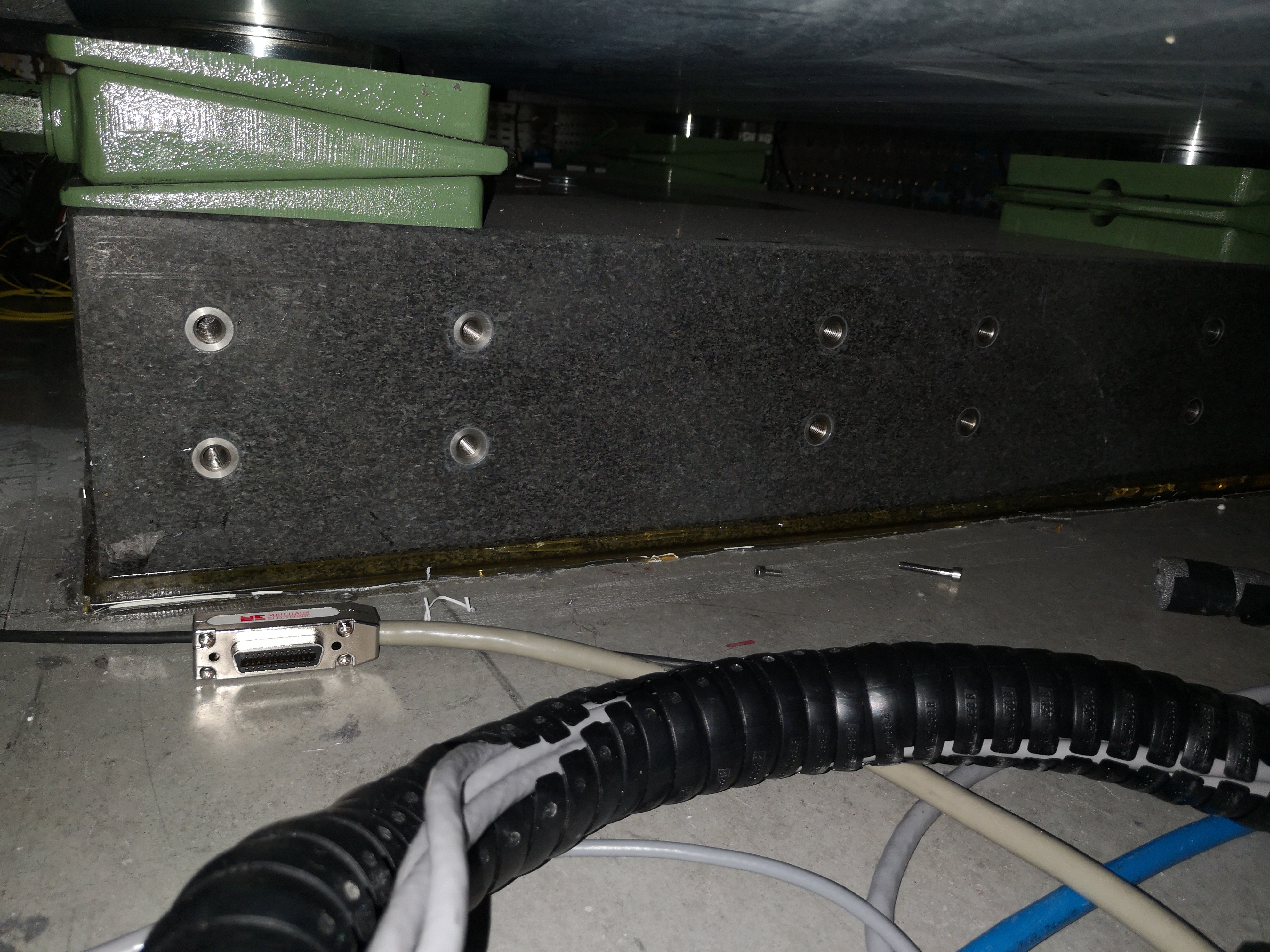
Figure 33: AirLoc used for the granite (2120-KSKC)
They are probably not well leveled so that could explain the first modes at 11Hz and 17Hz.
