Measurements on the instrumentation
Table of Contents
1 Measure of the noise of the Voltage Amplifier
The data and matlab files are accessible here.
1.1 Measurement Description
Goal:
- Determine the Voltage Amplifier noise
Setup:
- The two inputs (differential) of the voltage amplifier are shunted with 50Ohms
- The AC/DC option of the Voltage amplifier is on AC
- The low pass filter is set to 1hHz
- We measure the output of the voltage amplifier with a 16bits ADC of the Speedgoat
Measurements:
data_003: Ampli OFFdata_004: Ampli ON set to 20dBdata_005: Ampli ON set to 40dBdata_006: Ampli ON set to 60dB
1.2 Load data
amp_off = load('mat/data_003.mat', 'data'); amp_off = amp_off.data(:, [1,3]);
amp_20d = load('mat/data_004.mat', 'data'); amp_20d = amp_20d.data(:, [1,3]);
amp_40d = load('mat/data_005.mat', 'data'); amp_40d = amp_40d.data(:, [1,3]);
amp_60d = load('mat/data_006.mat', 'data'); amp_60d = amp_60d.data(:, [1,3]);
1.3 Time Domain
The time domain signals are shown on figure 1.
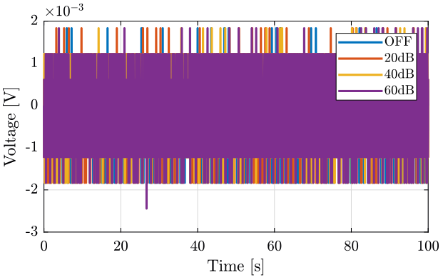
Figure 1: Output of the amplifier
1.4 Frequency Domain
We first compute some parameters that will be used for the PSD computation.
dt = amp_off(2, 2)-amp_off(1, 2);

Fs = 1/dt; % [Hz]

win = hanning(ceil(10*Fs));
Then we compute the Power Spectral Density using pwelch function.
[pxoff, f] = pwelch(amp_off(:,1), win, [], [], Fs);
[px20d, ~] = pwelch(amp_20d(:,1), win, [], [], Fs);
[px40d, ~] = pwelch(amp_40d(:,1), win, [], [], Fs);
[px60d, ~] = pwelch(amp_60d(:,1), win, [], [], Fs);
We compute the theoretical ADC noise.
q = 20/2^16; % quantization
Sq = q^2/12/1000; % PSD of the ADC noise
Finally, the ASD is shown on figure 2.
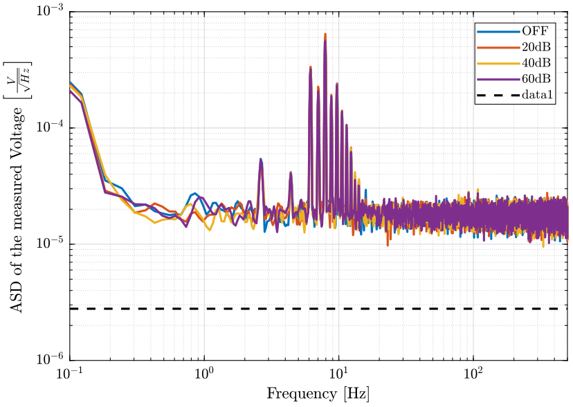
Figure 2: Amplitude Spectral Density of the measured voltage at the output of the voltage amplifier
1.5 Conclusion
Questions:
- Where does those sharp peaks comes from? Can this be due to aliasing?
Noise induced by the voltage amplifiers seems not to be a limiting factor as we have the same noise when they are OFF and ON.
2 Measure of the influence of the AC/DC option on the voltage amplifiers
The data and matlab files are accessible here.
2.1 Measurement Description
Goal:
- Measure the influence of the high-pass filter option of the voltage amplifiers
Setup:
- One geophone is located on the marble.
- It's signal goes to two voltage amplifiers with a gain of 60dB.
- One voltage amplifier is on the AC option, the other is on the DC option.
Measurements:
First measurement (mat/data_014.mat file):
| Column | Signal |
|---|---|
| 1 | Amplifier 1 with AC option |
| 2 | Amplifier 2 with DC option |
| 3 | Time |
Second measurement (mat/data_015.mat file):
| Column | Signal |
|---|---|
| 1 | Amplifier 1 with DC option |
| 2 | Amplifier 2 with AC option |
| 3 | Time |
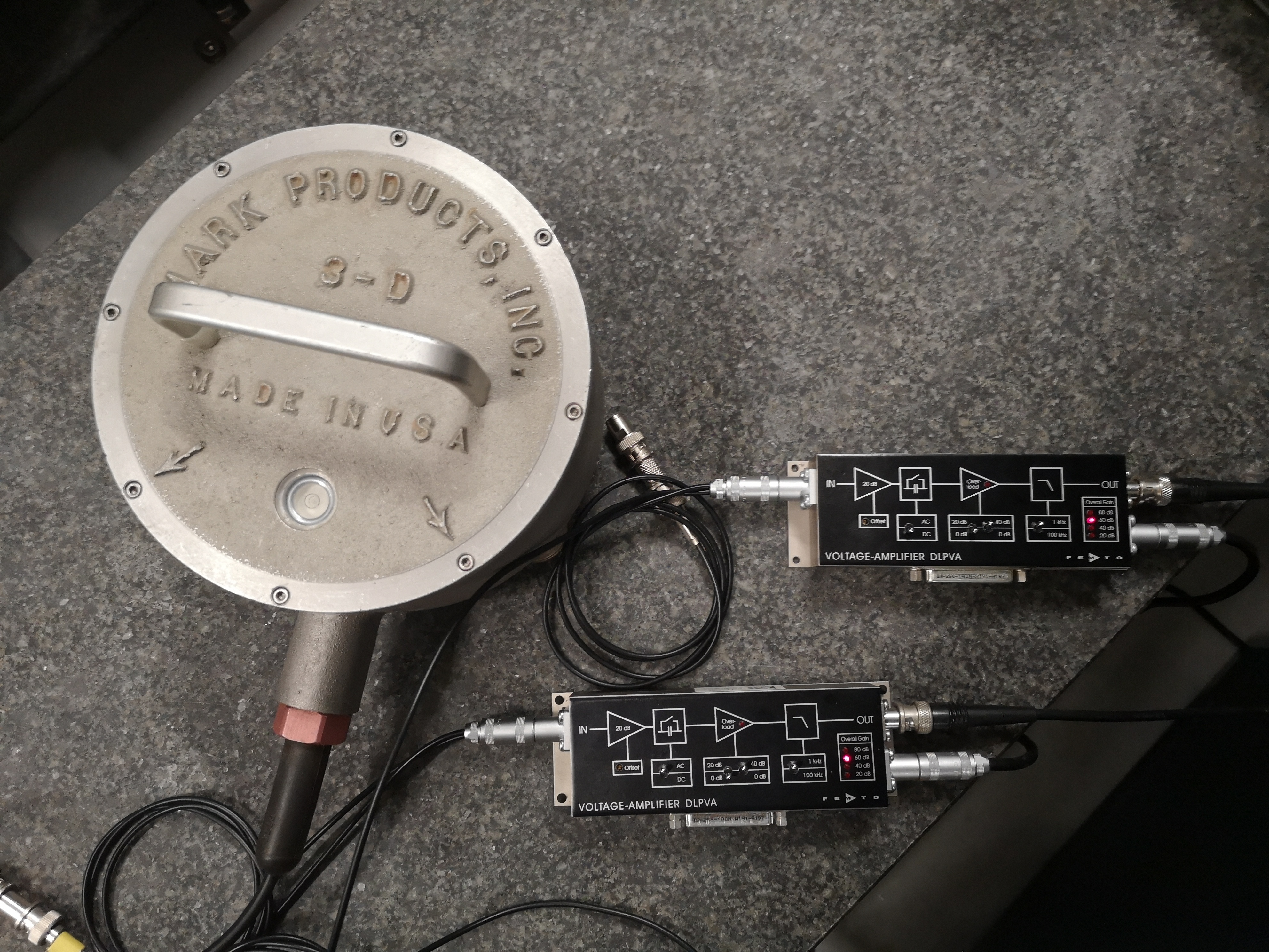
Figure 3: Picture of the two voltages amplifiers
2.2 Load data
We load the data of the z axis of two geophones.
meas14 = load('mat/data_014.mat', 'data'); meas14 = meas14.data;
meas15 = load('mat/data_015.mat', 'data'); meas15 = meas15.data;
2.3 Time Domain
The signals are shown on figure 4.
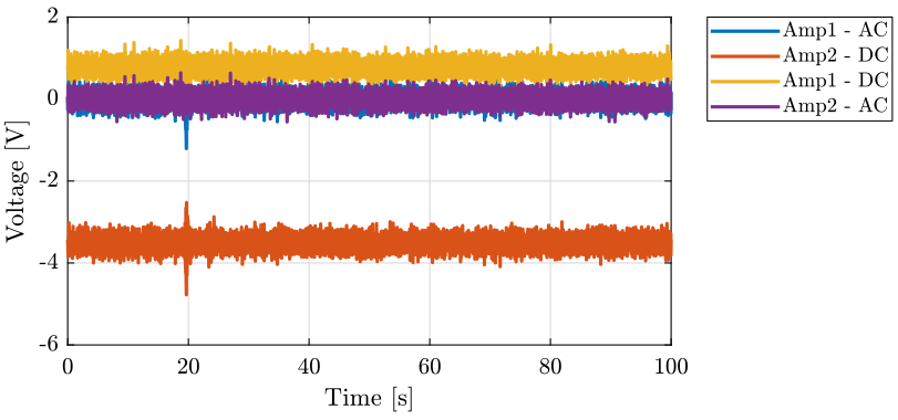
Figure 4: Comparison of the signals going through the Voltage amplifiers
2.4 Frequency Domain
We first compute some parameters that will be used for the PSD computation.
dt = meas14(2, 3)-meas14(1, 3);

Fs = 1/dt; % [Hz]

win = hanning(ceil(10*Fs));
Then we compute the Power Spectral Density using pwelch function.
[pxamp1ac, f] = pwelch(meas14(:, 1), win, [], [], Fs);
[pxamp2dc, ~] = pwelch(meas14(:, 2), win, [], [], Fs);

[pxamp1dc, ~] = pwelch(meas15(:, 1), win, [], [], Fs);
[pxamp2ac, ~] = pwelch(meas15(:, 2), win, [], [], Fs);
The ASD of the signals are compare on figure 5.
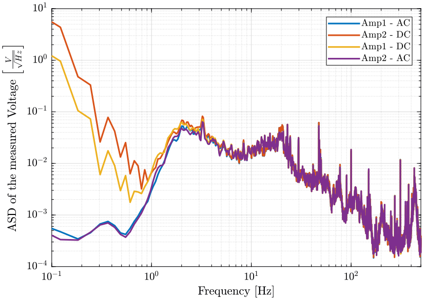
Figure 5: Amplitude Spectral Density of the measured signals
2.5 Conclusion
- The voltage amplifiers include some very sharp high pass filters at 1.5Hz (maybe 4th order)
- There is a DC offset on the time domain signal because the DC-offset knob was not set to zero
3 Transfer function of the Low Pass Filter
The computation files for this section are accessible here.
3.1 First LPF with a Cut-off frequency of 160Hz
3.1.1 Measurement Description
Goal:
- Measure the Low Pass Filter Transfer Function
The values of the components are:
\begin{aligned} R &= 1k\Omega \\ C &= 1\mu F \end{aligned}Which makes a cut-off frequency of \(f_c = \frac{1}{RC} = 1000 rad/s = 160Hz\).
\begin{tikzpicture}
  \draw (0,2)
        to [R=\(R\)] ++(2,0) node[circ]
        to ++(2,0)
        ++(-2,0)
        to [C=\(C\)] ++(0,-2) node[circ]
        ++(-2,0)
        to ++(2,0)
        to ++(2,0)
\end{tikzpicture}

Figure 6: Schematic of the Low Pass Filter used
Setup:
- We are measuring the signal from from Geophone with a BNC T
- On part goes to column 1 through the LPF
- The other part goes to column 2 without the LPF
Measurements:
mat/data_018.mat:
| Column | Signal |
|---|---|
| 1 | Amplifier 1 with LPF |
| 2 | Amplifier 2 |
| 3 | Time |
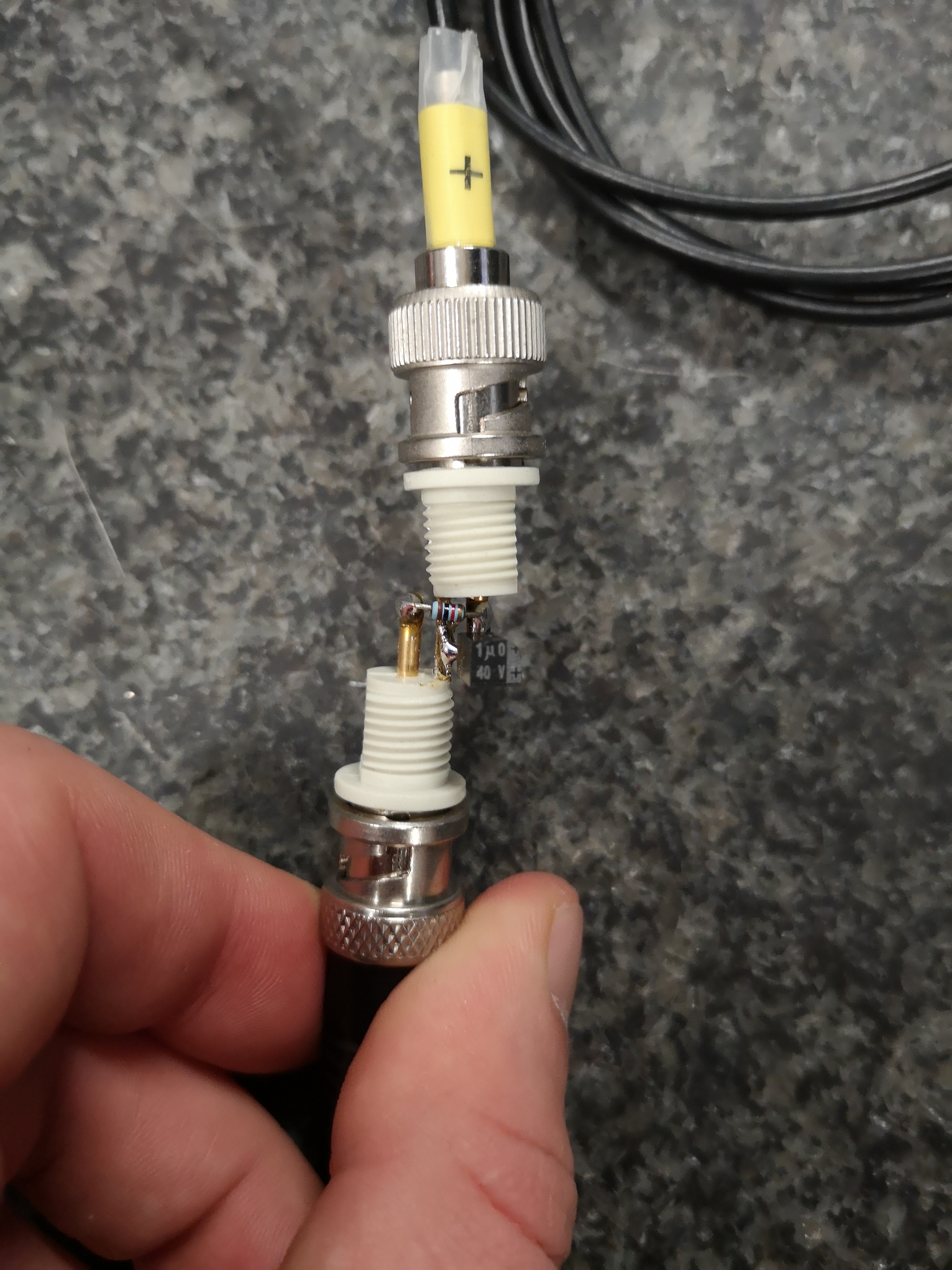
Figure 7: Picture of the low pass filter used
3.1.2 Load data
We load the data of the z axis of two geophones.
data = load('mat/data_018.mat', 'data'); data = data.data;
3.1.3 Transfer function of the LPF
We compute the transfer function from the signal without the LPF to the signal measured with the LPF.
dt = data(2, 3)-data(1, 3);

Fs = 1/dt; % [Hz]

win = hanning(ceil(10*Fs));
[Glpf, f] = tfestimate(data(:, 2), data(:, 1), win, [], [], Fs);
We compare this transfer function with a transfer function corresponding to an ideal first order LPF with a cut-off frequency of \(1000rad/s\). We obtain the result on figure 8.
Gth = 1/(1+s/1000)
figure;
ax1 = subplot(2, 1, 1);
hold on;
plot(f, abs(Glpf));
plot(f, abs(squeeze(freqresp(Gth, f, 'Hz'))));
hold off;
set(gca, 'xscale', 'log'); set(gca, 'yscale', 'log');
set(gca, 'XTickLabel',[]);
ylabel('Magnitude');

ax2 = subplot(2, 1, 2);
hold on;
plot(f, mod(180+180/pi*phase(Glpf), 360)-180);
plot(f, 180/pi*unwrap(angle(squeeze(freqresp(Gth, f, 'Hz')))));
hold off;
set(gca, 'xscale', 'log');
ylim([-180, 180]);
yticks([-180, -90, 0, 90, 180]);
xlabel('Frequency [Hz]'); ylabel('Phase');

linkaxes([ax1,ax2],'x');
xlim([1, 500]);
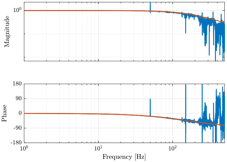
Figure 8: Bode Diagram of the measured Low Pass filter and the theoritical one
3.1.4 Conclusion
As we want to measure things up to \(500Hz\), we chose to change the value of the capacitor to obtain a cut-off frequency of \(1kHz\).
3.2 Second LPF with a Cut-off frequency of 1000Hz
3.2.1 Measurement description
This time, the value are
\begin{aligned} R &= 1k\Omega \\ C &= 150nF \end{aligned}Which makes a low pass filter with a cut-off frequency of \(f_c = 1060Hz\).
3.2.2 Load data
We load the data of the z axis of two geophones.
data = load('mat/data_019.mat', 'data'); data = data.data;
3.2.3 Transfer function of the LPF
We compute the transfer function from the signal without the LPF to the signal measured with the LPF.
dt = data(2, 3)-data(1, 3);

Fs = 1/dt; % [Hz]

win = hanning(ceil(10*Fs));
[Glpf, f] = tfestimate(data(:, 2), data(:, 1), win, [], [], Fs);
We compare this transfer function with a transfer function corresponding to an ideal first order LPF with a cut-off frequency of \(1060Hz\). We obtain the result on figure 9.
Gth = 1/(1+s/1060/2/pi);
figure;
ax1 = subplot(2, 1, 1);
hold on;
plot(f, abs(Glpf));
plot(f, abs(squeeze(freqresp(Gth, f, 'Hz'))));
hold off;
set(gca, 'xscale', 'log'); set(gca, 'yscale', 'log');
set(gca, 'XTickLabel',[]);
ylabel('Magnitude');

ax2 = subplot(2, 1, 2);
hold on;
plot(f, mod(180+180/pi*phase(Glpf), 360)-180);
plot(f, 180/pi*unwrap(angle(squeeze(freqresp(Gth, f, 'Hz')))));
hold off;
set(gca, 'xscale', 'log');
ylim([-180, 180]);
yticks([-180, -90, 0, 90, 180]);
xlabel('Frequency [Hz]'); ylabel('Phase');

linkaxes([ax1,ax2],'x');
xlim([1, 500]);
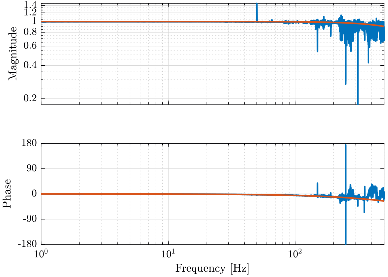
Figure 9: Bode Diagram of the measured Low Pass filter and the theoritical one
3.2.4 Conclusion
The added LPF has the expected behavior.