Vibrations induced by the Slip-Ring and the Spindle

1. Experimental Setup
2. Data Analysis

1 Experimental Setup

Setup: One geophone is located on the marble, the other one on the floor (see figure 1).

Two geophone are use:

One on the floor (corresponding to the first column in the data)
One at the marble location (corresponding to the second column in the data)

Two voltage amplifiers are used, their setup is:

gain of 60dB
AC/DC switch on AC
Low pass filter at 1kHz

A first order low pass filter is also added at the input of the voltage amplifiers.

Goal:

Identify the marble dynamics in all the directions

Measurements: Three measurements are done:

Measurement File	Description
`mat/data_037.mat`	Z direction
`mat/data_038.mat`	N direction
`mat/data_039.mat`	E direction

Each of the measurement mat file contains one data array with 3 columns:

Column number	Description
1	Geophone - Floor
2	Geophone - Marble
3	Time

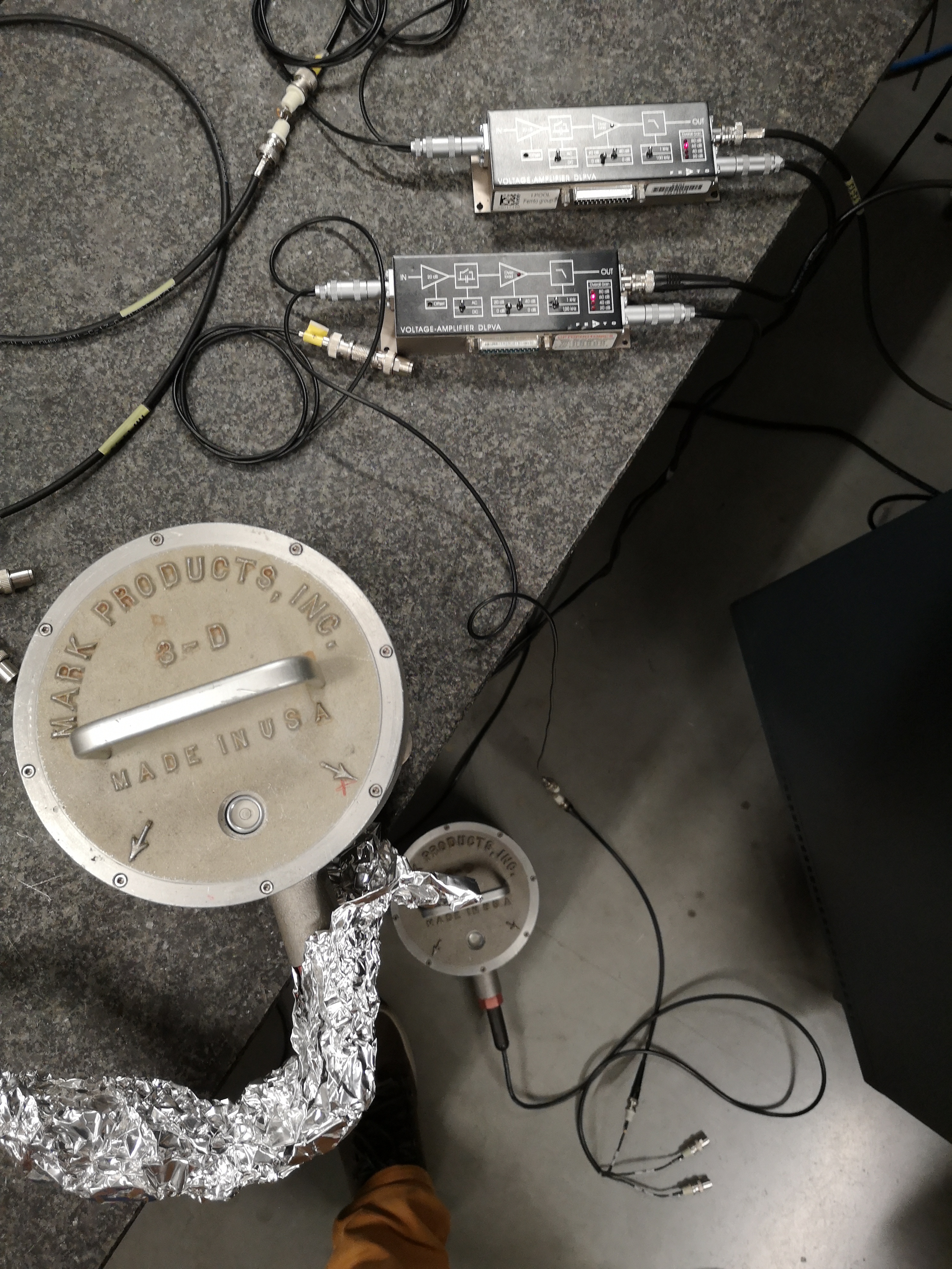
Figure 1: Picture of the experimental setup

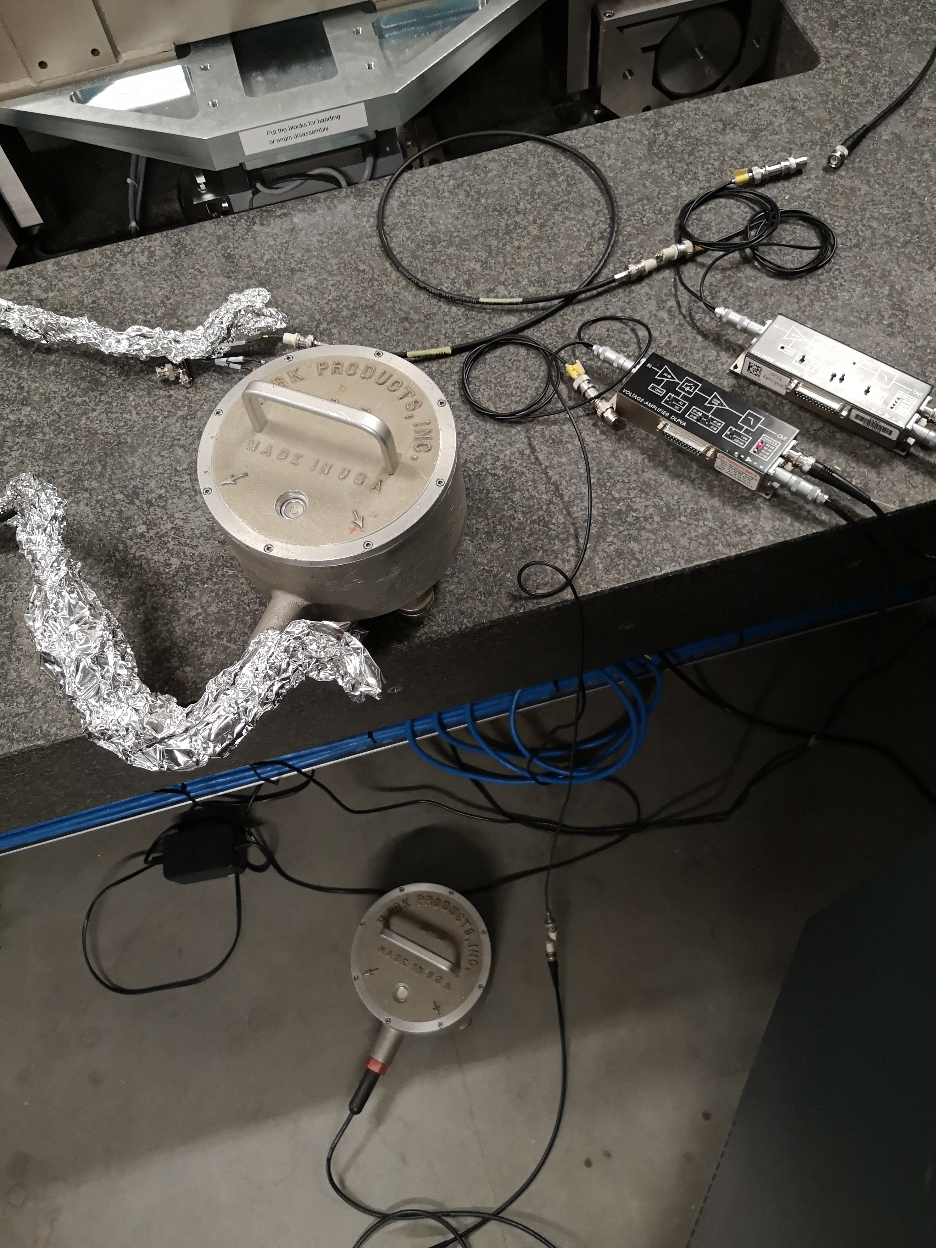
Figure 2: Picture of the experimental setup

2 Data Analysis

All the files (data and Matlab scripts) are accessible here.

2.1 Load data

m_z = load('mat/data_037.mat', 'data'); m_z = m_z.data;
m_n = load('mat/data_038.mat', 'data'); m_n = m_n.data;
m_e = load('mat/data_039.mat', 'data'); m_e = m_e.data;

2.2 Time domain plots

figure;
subplot(1, 3, 1);
hold on;
plot(m_z(:, 3), m_z(:, 2), 'DisplayName', 'Marble - Z');
plot(m_z(:, 3), m_z(:, 1), 'DisplayName', 'Floor - Z');
hold off;
xlabel('Time [s]'); ylabel('Voltage [V]');
xlim([0, 100]); ylim([-2 2]);
legend('Location', 'northeast');

subplot(1, 3, 2);
hold on;
plot(m_n(:, 3), m_n(:, 2), 'DisplayName', 'Marble - N');
plot(m_n(:, 3), m_n(:, 1), 'DisplayName', 'Floor - N');
hold off;
xlabel('Time [s]'); ylabel('Voltage [V]');
xlim([0, 100]); ylim([-2 2]);
legend('Location', 'northeast');

subplot(1, 3, 3);
hold on;
plot(m_e(:, 3), m_e(:, 2), 'DisplayName', 'Marble - E');
plot(m_e(:, 3), m_e(:, 1), 'DisplayName', 'Floor - E');
hold off;
xlabel('Time [s]'); ylabel('Voltage [V]');
xlim([0, 100]); ylim([-2 2]);
legend('Location', 'northeast');

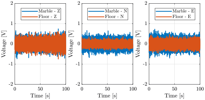
Figure 3: Floor and ground motion

2.3 Compute the power spectral densities

We first compute some parameters that will be used for the PSD computation.

dt = m_z(2, 3)-m_z(1, 3);

Fs = 1/dt; % [Hz]

win = hanning(ceil(10*Fs));

Then we compute the Power Spectral Density using pwelch function.

[px_fz, f] = pwelch(m_z(:, 1), win, [], [], Fs);
[px_gz, ~] = pwelch(m_z(:, 2), win, [], [], Fs);

[px_fn, ~] = pwelch(m_n(:, 1), win, [], [], Fs);
[px_gn, ~] = pwelch(m_n(:, 2), win, [], [], Fs);

[px_fe, ~] = pwelch(m_e(:, 1), win, [], [], Fs);
[px_ge, ~] = pwelch(m_e(:, 2), win, [], [], Fs);

The results are shown on figure 4 for the Z direction, figure 5 for the north direction, and figure 6 for the east direction.

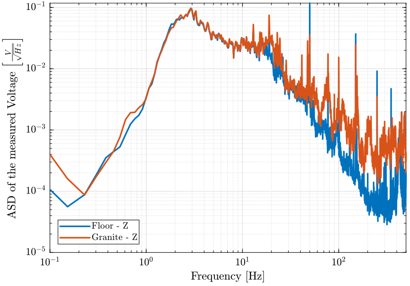
Figure 4: Amplitude Spectral Density of the measured voltage corresponding to the geophone located on the floor and on the marble - Z direction

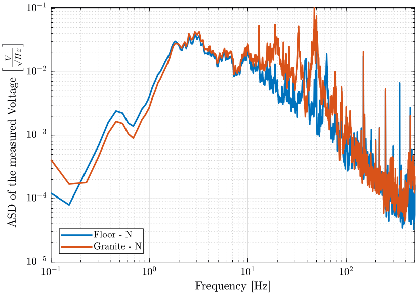
Figure 5: Amplitude Spectral Density of the measured voltage corresponding to the geophone located on the floor and on the marble - N direction

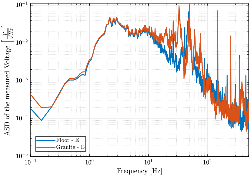
Figure 6: Amplitude Spectral Density of the measured voltage corresponding to the geophone located on the floor and on the marble - E direction

2.4 Compute the transfer function from floor motion to ground motion

We now compute the transfer function from the floor motion to the granite motion.

The result is shown on figure 7.

[TZ, f] = tfestimate(m_z(:, 1), -m_z(:, 2), win, [], [], Fs);
[TN, ~] = tfestimate(m_n(:, 1), -m_n(:, 2), win, [], [], Fs);
[TE, ~] = tfestimate(m_e(:, 1), -m_e(:, 2), win, [], [], Fs);

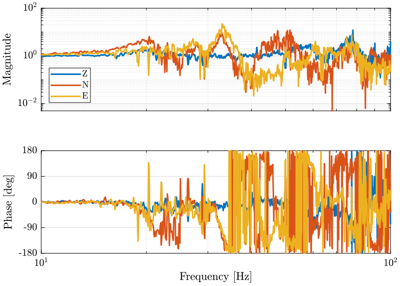
Figure 7: Transfer function from floor motion to granite motion

2.5 Conclusion

We see resonance of the granite at 33Hz in the horizontal directions
We see two resonances for the z direction: at 60Hz and 75Hz