Effect on the control system of each stages on the vibration of the station

1. Effect of all the control systems on the Sample vibrations
2. Effect of all the control systems on the Sample vibrations - One stage at a time
3. Effect of the Symetrie Driver

This file is organized as follow:

Section 1:
- One geophone on the marble and one at the sample location
- Each stage is turned on one by one
Section 2:
- One geophone on the marble and one at the sample location
- Each stage is turned on one at a time
Section 3:
- We check if the Symetrie driver induces some vibrations when placed on the marble

1 Effect of all the control systems on the Sample vibrations

All the files (data and Matlab scripts) are accessible here.

1.1 Experimental Setup

We here measure the signals of two L22 geophones:

One is located on top of the Sample platform
One is located on the marble

The signals are amplified with voltage amplifiers with the following settings:

gain of 60dB
AC/DC option set on AC
Low pass filter set at 1kHz

The signal from the top geophone does not go trought the slip-ring.

First, all the control systems are turned ON, then, they are turned one by one. Each measurement are done during 50s.

Table 1: Summary of the measurements and the states of the control systems
Ty	Ry	Slip Ring	Spindle	Hexapod	Meas. file
ON	ON	ON	ON	ON	`meas_003.mat`
OFF	ON	ON	ON	ON	`meas_004.mat`
OFF	OFF	ON	ON	ON	`meas_005.mat`
OFF	OFF	OFF	ON	ON	`meas_006.mat`
OFF	OFF	OFF	OFF	ON	`meas_007.mat`
OFF	OFF	OFF	OFF	OFF	`meas_008.mat`

Each of the mat file contains one array data with 3 columns:

Column number	Description
1	Geophone - Marble
2	Geophone - Sample
3	Time

1.2 Load data

We load the data of the z axis of two geophones.

d3 = load('mat/data_003.mat', 'data'); d3 = d3.data;
d4 = load('mat/data_004.mat', 'data'); d4 = d4.data;
d5 = load('mat/data_005.mat', 'data'); d5 = d5.data;
d6 = load('mat/data_006.mat', 'data'); d6 = d6.data;
d7 = load('mat/data_007.mat', 'data'); d7 = d7.data;
d8 = load('mat/data_008.mat', 'data'); d8 = d8.data;

1.3 Analysis - Time Domain

First, we can look at the time domain data and compare all the measurements:

comparison for the geophone at the sample location (figure 1)
comparison for the geophone on the granite (figure 2)

figure;
hold on;
plot(d3(:, 3), d3(:, 2), 'DisplayName', 'Hexa, Rz, SR, Ry, Ty');
plot(d4(:, 3), d4(:, 2), 'DisplayName', 'Hexa, Rz, SR, Ry');
plot(d5(:, 3), d5(:, 2), 'DisplayName', 'Hexa, Rz, SR');
plot(d6(:, 3), d6(:, 2), 'DisplayName', 'Hexa, Rz');
plot(d7(:, 3), d7(:, 2), 'DisplayName', 'Hexa');
plot(d8(:, 3), d8(:, 2), 'DisplayName', 'All OFF');
hold off;
xlabel('Time [s]'); ylabel('Voltage [V]');
xlim([0, 50]);
legend('Location', 'bestoutside');

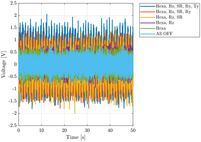
Figure 1: Comparison of the time domain data when turning off the control system of the stages - Geophone at the sample location

figure;
hold on;
plot(d3(:, 3), d3(:, 1), 'DisplayName', 'Hexa, Rz, SR, Ry, Ty');
plot(d4(:, 3), d4(:, 1), 'DisplayName', 'Hexa, Rz, SR, Ry');
plot(d5(:, 3), d5(:, 1), 'DisplayName', 'Hexa, Rz, SR');
plot(d6(:, 3), d6(:, 1), 'DisplayName', 'Hexa, Rz');
plot(d7(:, 3), d7(:, 1), 'DisplayName', 'Hexa');
plot(d8(:, 3), d8(:, 1), 'DisplayName', 'All OFF');
hold off;
xlabel('Time [s]'); ylabel('Voltage [V]');
xlim([0, 50]);
legend('Location', 'bestoutside');

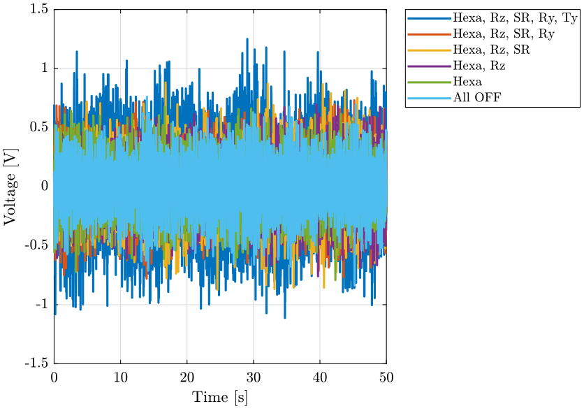
Figure 2: Comparison of the time domain data when turning off the control system of the stages - Geophone on the marble

1.4 Analysis - Frequency Domain

dt = d3(2, 3) - d3(1, 3);

Fs = 1/dt;
win = hanning(ceil(10*Fs));

1.4.1 Vibrations at the sample location

First, we compute the Power Spectral Density of the signals coming from the Geophone located at the sample location.

[px3, f] = pwelch(d3(:, 2), win, [], [], Fs);
[px4, ~] = pwelch(d4(:, 2), win, [], [], Fs);
[px5, ~] = pwelch(d5(:, 2), win, [], [], Fs);
[px6, ~] = pwelch(d6(:, 2), win, [], [], Fs);
[px7, ~] = pwelch(d7(:, 2), win, [], [], Fs);
[px8, ~] = pwelch(d8(:, 2), win, [], [], Fs);

And we compare all the signals (figures 3 and 4).

figure;
hold on;
plot(f, sqrt(px3), 'DisplayName', 'Hexa, Rz, SR, Ry, Ty');
plot(f, sqrt(px4), 'DisplayName', 'Hexa, Rz, SR, Ry');
plot(f, sqrt(px5), 'DisplayName', 'Hexa, Rz, SR');
plot(f, sqrt(px6), 'DisplayName', 'Hexa, Rz');
plot(f, sqrt(px7), 'DisplayName', 'Hexa');
plot(f, sqrt(px8), 'DisplayName', 'All OFF');
plot(fgm, sqrt(pxxgm), '-k', 'DisplayName', 'Ground Velocity');
hold off;
set(gca, 'xscale', 'log');
set(gca, 'yscale', 'log');
xlabel('Frequency [Hz]'); ylabel('Amplitude Spectral Density $\left[\frac{V}{\sqrt{Hz}}\right]$')
xlim([0.1, 500]);
legend('Location', 'southwest');

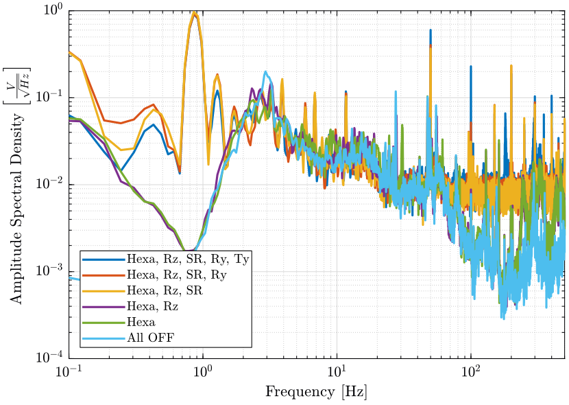
Figure 3: Amplitude Spectral Density of the signal coming from the top geophone

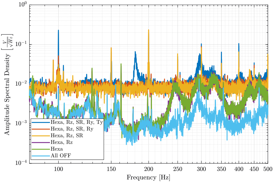
Figure 4: Amplitude Spectral Density of the signal coming from the top geophone (zoom at high frequencies)

1.4.2 Vibrations on the marble

Now we plot the same curves for the geophone located on the marble.

[px3, f] = pwelch(d3(:, 1), win, [], [], Fs);
[px4, ~] = pwelch(d4(:, 1), win, [], [], Fs);
[px5, ~] = pwelch(d5(:, 1), win, [], [], Fs);
[px6, ~] = pwelch(d6(:, 1), win, [], [], Fs);
[px7, ~] = pwelch(d7(:, 1), win, [], [], Fs);
[px8, ~] = pwelch(d8(:, 1), win, [], [], Fs);

And we compare the Amplitude Spectral Densities (figures 5 and 6)

figure;
hold on;
plot(f, sqrt(px3), 'DisplayName', 'Hexa, Rz, SR, Ry, Ty');
plot(f, sqrt(px4), 'DisplayName', 'Hexa, Rz, SR, Ry');
plot(f, sqrt(px5), 'DisplayName', 'Hexa, Rz, SR');
plot(f, sqrt(px6), 'DisplayName', 'Hexa, Rz');
plot(f, sqrt(px7), 'DisplayName', 'Hexa');
plot(f, sqrt(px8), 'DisplayName', 'All OFF');
plot(fgm, sqrt(pxxgm), '-k', 'DisplayName', 'Ground Velocity');
hold off;
set(gca, 'xscale', 'log');
set(gca, 'yscale', 'log');
xlabel('Frequency [Hz]'); ylabel('Amplitude Spectral Density $\left[\frac{V}{\sqrt{Hz}}\right]$')
xlim([0.1, 500]);
legend('Location', 'northeast');

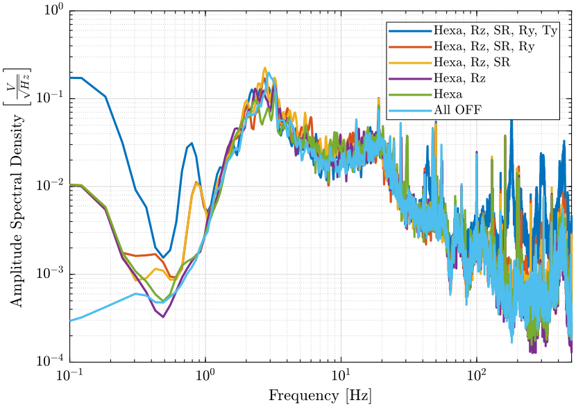
Figure 5: Amplitude Spectral Density of the signal coming from the top geophone

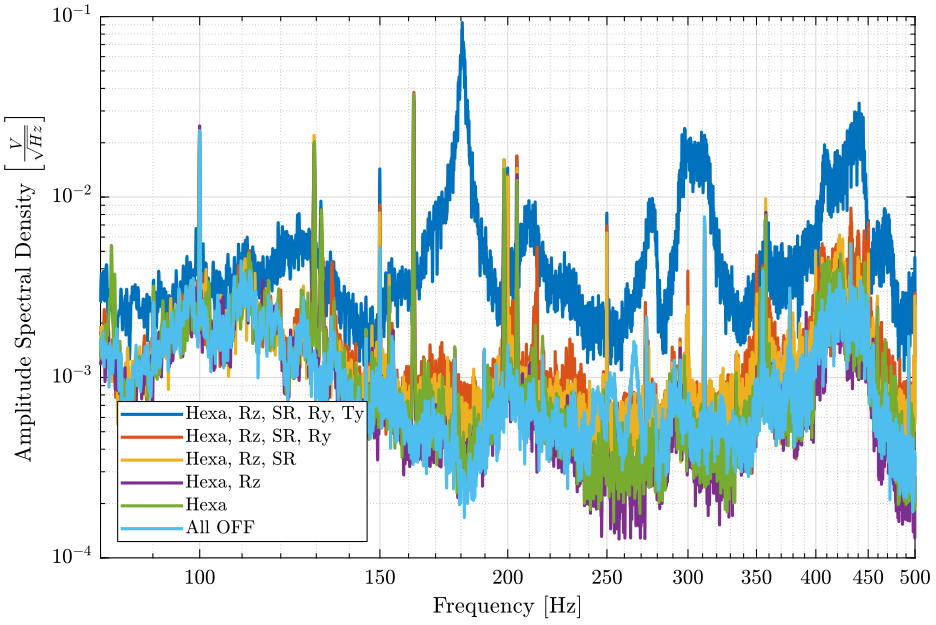
Figure 6: Amplitude Spectral Density of the signal coming from the top geophone (zoom at high frequencies)

1.5 Conclusion

The control system of the Ty stage induces a lot of vibrations of the marble

2 Effect of all the control systems on the Sample vibrations - One stage at a time

All the files (data and Matlab scripts) are accessible here.

2.1 Experimental Setup

We here measure the signals of two geophones:

One is located on top of the Sample platform
One is located on the marble

The signal from the top geophone does go trought the slip-ring.

All the control systems are turned OFF, then, they are turned on one at a time.

Each measurement are done during 100s.

The settings of the voltage amplifier are shown on figure 7:

gain of 60dB
AC/DC option set on DC
Low pass filter set at 1kHz

A first order low pass filter with a cut-off frequency of 1kHz is added before the voltage amplifier.

Table 2: Summary of the measurements and the states of the control systems
Ty	Ry	Slip Ring	Spindle	Hexapod	Meas. file
OFF	OFF	OFF	OFF	OFF	`meas_013.mat`
ON	OFF	OFF	OFF	OFF	`meas_014.mat`
OFF	ON	OFF	OFF	OFF	`meas_015.mat`
OFF	OFF	ON	OFF	OFF	`meas_016.mat`
OFF	OFF	OFF	ON	OFF	`meas_017.mat`
OFF	OFF	OFF	OFF	ON	`meas_018.mat`

Each of the mat file contains one array data with 3 columns:

Column number	Description
1	Geophone - Marble
2	Geophone - Sample
3	Time

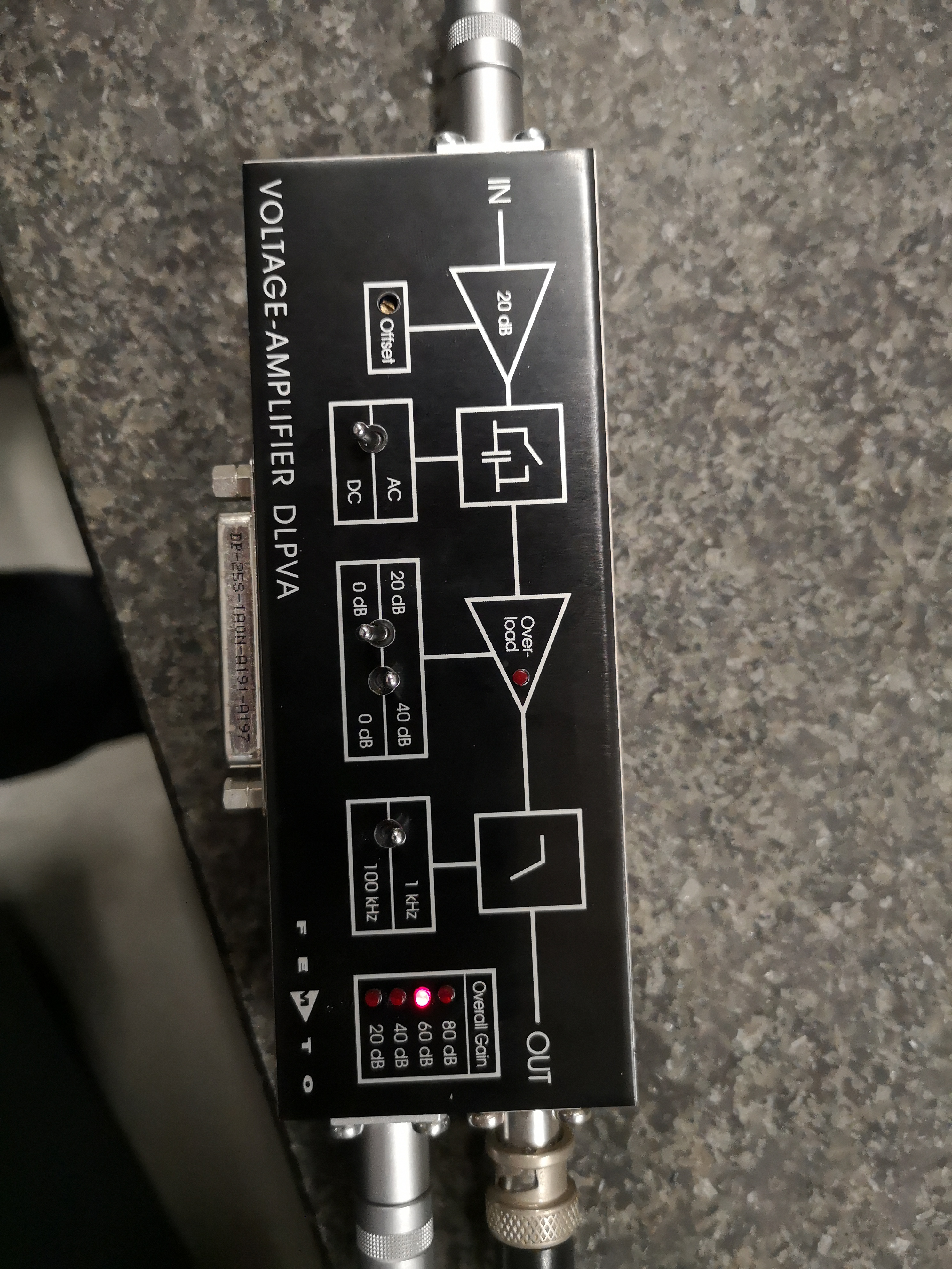
Figure 7: Voltage amplifier settings for the measurement

2.2 Load data

We load the data of the z axis of two geophones.

d_of = load('mat/data_013.mat', 'data'); d_of = d_of.data;
d_ty = load('mat/data_014.mat', 'data'); d_ty = d_ty.data;
d_ry = load('mat/data_015.mat', 'data'); d_ry = d_ry.data;
d_sr = load('mat/data_016.mat', 'data'); d_sr = d_sr.data;
d_rz = load('mat/data_017.mat', 'data'); d_rz = d_rz.data;
d_he = load('mat/data_018.mat', 'data'); d_he = d_he.data;

2.3 Voltage to Velocity

We convert the measured voltage to velocity using the function voltageToVelocityL22 (accessible here).

gain = 60; % [dB]

d_of(:, 1) = voltageToVelocityL22(d_of(:, 1), d_of(:, 3), gain);
d_ty(:, 1) = voltageToVelocityL22(d_ty(:, 1), d_ty(:, 3), gain);
d_ry(:, 1) = voltageToVelocityL22(d_ry(:, 1), d_ry(:, 3), gain);
d_sr(:, 1) = voltageToVelocityL22(d_sr(:, 1), d_sr(:, 3), gain);
d_rz(:, 1) = voltageToVelocityL22(d_rz(:, 1), d_rz(:, 3), gain);
d_he(:, 1) = voltageToVelocityL22(d_he(:, 1), d_he(:, 3), gain);

d_of(:, 2) = voltageToVelocityL22(d_of(:, 2), d_of(:, 3), gain);
d_ty(:, 2) = voltageToVelocityL22(d_ty(:, 2), d_ty(:, 3), gain);
d_ry(:, 2) = voltageToVelocityL22(d_ry(:, 2), d_ry(:, 3), gain);
d_sr(:, 2) = voltageToVelocityL22(d_sr(:, 2), d_sr(:, 3), gain);
d_rz(:, 2) = voltageToVelocityL22(d_rz(:, 2), d_rz(:, 3), gain);
d_he(:, 2) = voltageToVelocityL22(d_he(:, 2), d_he(:, 3), gain);

2.4 Analysis - Time Domain

First, we can look at the time domain data and compare all the measurements:

comparison for the geophone at the sample location (figure 8)
comparison for the geophone on the granite (figure 9)
relative displacement of the sample with respect to the marble (figure 9)

figure;
hold on;
plot(d_of(:, 3), d_of(:, 2), 'DisplayName', 'All OFF');
plot(d_ty(:, 3), d_ty(:, 2), 'DisplayName', 'Ty ON');
plot(d_ry(:, 3), d_ry(:, 2), 'DisplayName', 'Ry ON');
plot(d_sr(:, 3), d_sr(:, 2), 'DisplayName', 'S-R ON');
plot(d_rz(:, 3), d_rz(:, 2), 'DisplayName', 'Rz ON');
plot(d_he(:, 3), d_he(:, 2), 'DisplayName', 'Hexa ON');
hold off;
xlabel('Time [s]'); ylabel('Velocity [m/s]');
xlim([0, 50]);
legend('Location', 'bestoutside');

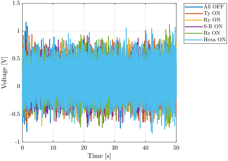
Figure 8: Comparison of the time domain data when turning off the control system of the stages - Geophone at the sample location

figure;
hold on;
plot(d_of(:, 3), d_of(:, 1), 'DisplayName', 'All OFF');
plot(d_ty(:, 3), d_ty(:, 1), 'DisplayName', 'Ty ON');
plot(d_ry(:, 3), d_ry(:, 1), 'DisplayName', 'Ry ON');
plot(d_sr(:, 3), d_sr(:, 1), 'DisplayName', 'S-R ON');
plot(d_rz(:, 3), d_rz(:, 1), 'DisplayName', 'Rz ON');
plot(d_he(:, 3), d_he(:, 1), 'DisplayName', 'Hexa ON');
hold off;
xlabel('Time [s]'); ylabel('Velocity [m/s]');
xlim([0, 50]);
legend('Location', 'bestoutside');

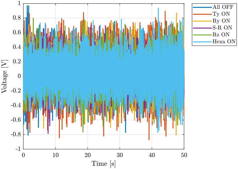
Figure 9: Comparison of the time domain data when turning off the control system of the stages - Geophone on the marble

figure;
hold on;
plot(d_of(:, 3), 1e6*lsim(1/(1+s/(2*pi*0.5)), d_of(:, 2)-d_of(:, 1), d_of(:, 3)), 'DisplayName', 'All OFF');
plot(d_ty(:, 3), 1e6*lsim(1/(1+s/(2*pi*0.5)), d_ty(:, 2)-d_ty(:, 1), d_ty(:, 3)), 'DisplayName', 'Ty ON');
plot(d_ry(:, 3), 1e6*lsim(1/(1+s/(2*pi*0.5)), d_ry(:, 2)-d_ry(:, 1), d_ry(:, 3)), 'DisplayName', 'Ry ON');
plot(d_sr(:, 3), 1e6*lsim(1/(1+s/(2*pi*0.5)), d_sr(:, 2)-d_sr(:, 1), d_sr(:, 3)), 'DisplayName', 'S-R ON');
plot(d_rz(:, 3), 1e6*lsim(1/(1+s/(2*pi*0.5)), d_rz(:, 2)-d_rz(:, 1), d_rz(:, 3)), 'DisplayName', 'Rz ON');
plot(d_he(:, 3), 1e6*lsim(1/(1+s/(2*pi*0.5)), d_he(:, 2)-d_he(:, 1), d_he(:, 3)), 'DisplayName', 'Hexa ON');
hold off;
xlabel('Time [s]'); ylabel('Relative Displacement [$\mu m$]');
xlim([0, 50]);
legend('Location', 'bestoutside');

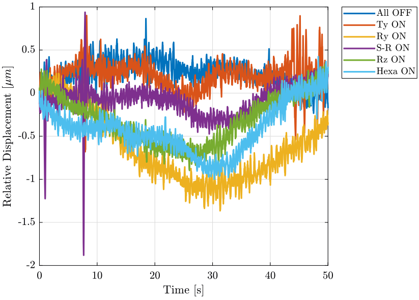
Figure 10: Relative displacement of the sample with respect to the marble

2.5 Analysis - Frequency Domain

dt = d_of(2, 3) - d_of(1, 3);

Fs = 1/dt;
win = hanning(ceil(10*Fs));

2.5.1 Vibrations at the sample location

First, we compute the Power Spectral Density of the signals coming from the Geophone located at the sample location.

[px_of, f] = pwelch(d_of(:, 2), win, [], [], Fs);
[px_ty, ~] = pwelch(d_ty(:, 2), win, [], [], Fs);
[px_ry, ~] = pwelch(d_ry(:, 2), win, [], [], Fs);
[px_sr, ~] = pwelch(d_sr(:, 2), win, [], [], Fs);
[px_rz, ~] = pwelch(d_rz(:, 2), win, [], [], Fs);
[px_he, ~] = pwelch(d_he(:, 2), win, [], [], Fs);

And we compare all the signals (figures 11 and 12).

figure;
hold on;
plot(f, sqrt(px_of), 'DisplayName', 'All OFF');
plot(f, sqrt(px_ty), 'DisplayName', 'Ty ON');
plot(f, sqrt(px_ry), 'DisplayName', 'Ry ON');
plot(f, sqrt(px_sr), 'DisplayName', 'S-R ON');
plot(f, sqrt(px_rz), 'DisplayName', 'Rz ON');
plot(f, sqrt(px_he), 'DisplayName', 'Hexa ON');
hold off;
set(gca, 'xscale', 'log');
set(gca, 'yscale', 'log');
xlabel('Frequency [Hz]'); ylabel('Amplitude Spectral Density $\left[\frac{m/s}{\sqrt{Hz}}\right]$')
xlim([0.1, 500]);
legend('Location', 'southwest');

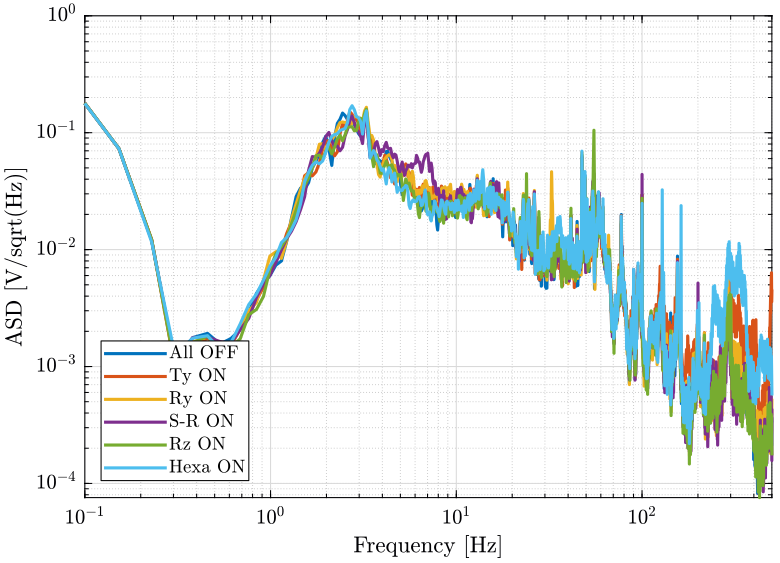
Figure 11: Amplitude Spectral Density of the sample velocity

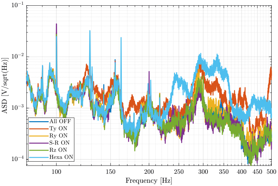
Figure 12: Amplitude Spectral Density of the sample velocity (zoom at high frequencies)

2.5.2 Vibrations on the marble

Now we plot the same curves for the geophone located on the marble.

[px_of, f] = pwelch(d_of(:, 1), win, [], [], Fs);
[px_ty, ~] = pwelch(d_ty(:, 1), win, [], [], Fs);
[px_ry, ~] = pwelch(d_ry(:, 1), win, [], [], Fs);
[px_sr, ~] = pwelch(d_sr(:, 1), win, [], [], Fs);
[px_rz, ~] = pwelch(d_rz(:, 1), win, [], [], Fs);
[px_he, ~] = pwelch(d_he(:, 1), win, [], [], Fs);

And we compare the Amplitude Spectral Densities (figures 13 and 14)

figure;
hold on;
plot(f, sqrt(px_of), 'DisplayName', 'All OFF');
plot(f, sqrt(px_ty), 'DisplayName', 'Ty ON');
plot(f, sqrt(px_ry), 'DisplayName', 'Ry ON');
plot(f, sqrt(px_sr), 'DisplayName', 'S-R ON');
plot(f, sqrt(px_rz), 'DisplayName', 'Rz ON');
plot(f, sqrt(px_he), 'DisplayName', 'Hexa ON');
hold off;
set(gca, 'xscale', 'log');
set(gca, 'yscale', 'log');
xlabel('Frequency [Hz]'); ylabel('Amplitude Spectral Density $\left[\frac{m/s}{\sqrt{Hz}}\right]$')
xlim([0.1, 500]);
legend('Location', 'northeast');

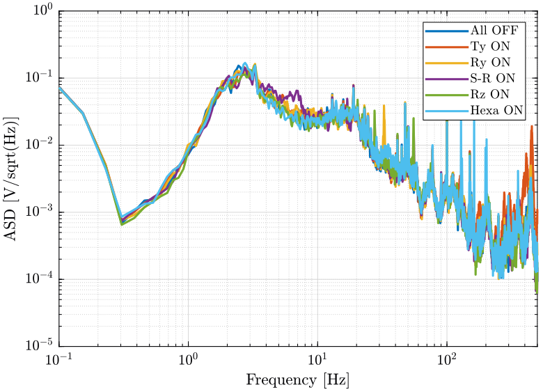
Figure 13: Amplitude Spectral Density of the marble velocity

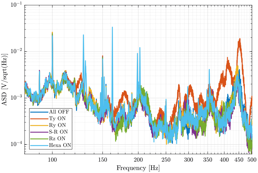
Figure 14: Amplitude Spectral Density of the marble velocity (zoom at high frequencies)

2.6 Conclusion

The Ty stage induces vibrations of the marble and at the sample location above 100Hz
The hexapod stage induces vibrations at the sample position above 220Hz

3 Effect of the Symetrie Driver

All the files (data and Matlab scripts) are accessible here.

3.1 Experimental Setup

We here measure the signals of two geophones:

One is located on top of the Sample platform
One is located on the marble

The signal from the top geophone does go trought the slip-ring.

All the control systems are turned OFF except the Hexapod one.

Each measurement are done during 100s.

The settings of the voltage amplifier are:

gain of 60dB
AC/DC option set on DC
Low pass filter set at 1kHz

A first order low pass filter with a cut-off frequency of 1kHz is added before the voltage amplifier.

The measurements are:

meas_018.mat: Hexapod's driver on the granite
meas_019.mat: Hexapod's driver on the ground

Each of the mat file contains one array data with 3 columns:

Column number	Description
1	Geophone - Marble
2	Geophone - Sample
3	Time

3.2 Load data

We load the data of the z axis of two geophones.

d_18 = load('mat/data_018.mat', 'data'); d_18 = d_18.data;
d_19 = load('mat/data_019.mat', 'data'); d_19 = d_19.data;

3.3 Analysis - Time Domain

figure;
hold on;
plot(d_19(:, 3), d_19(:, 1), 'DisplayName', 'Driver - Ground');
plot(d_18(:, 3), d_18(:, 1), 'DisplayName', 'Driver - Granite');
hold off;
xlabel('Time [s]'); ylabel('Voltage [V]');
xlim([0, 50]);
legend('Location', 'bestoutside');

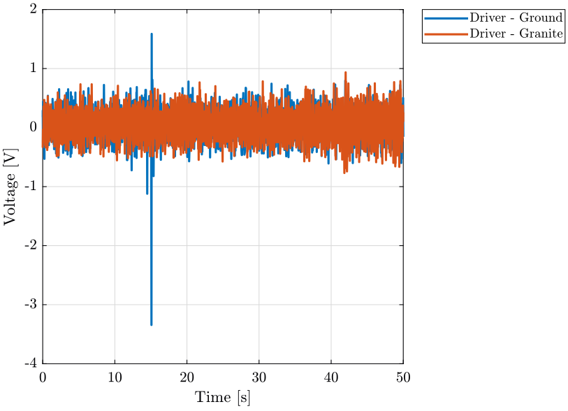
Figure 15: Comparison of the time domain data when turning off the control system of the stages - Geophone at the sample location

3.4 Analysis - Frequency Domain

dt = d_18(2, 3) - d_18(1, 3);

Fs = 1/dt;
win = hanning(ceil(10*Fs));

3.4.1 Vibrations at the sample location

First, we compute the Power Spectral Density of the signals coming from the Geophone located at the sample location.

[px_18, f] = pwelch(d_18(:, 1), win, [], [], Fs);
[px_19, ~] = pwelch(d_19(:, 1), win, [], [], Fs);

figure;
hold on;
plot(f, sqrt(px_19), 'DisplayName', 'Driver - Ground');
plot(f, sqrt(px_18), 'DisplayName', 'Driver - Granite');
hold off;
set(gca, 'xscale', 'log');
set(gca, 'yscale', 'log');
xlabel('Frequency [Hz]'); ylabel('Amplitude Spectral Density $\left[\frac{V}{\sqrt{Hz}}\right]$')
xlim([0.1, 500]);
legend('Location', 'southwest');

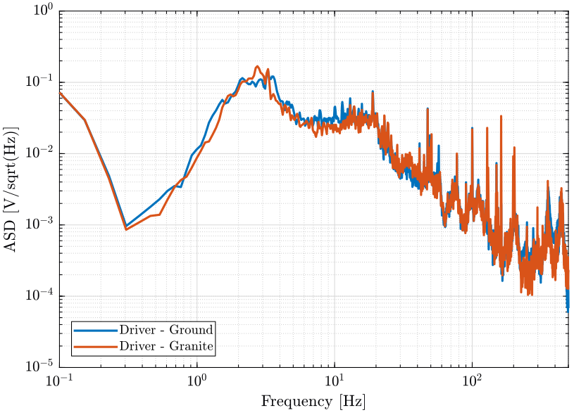
Figure 16: Amplitude Spectral Density of the signal coming from the top geophone

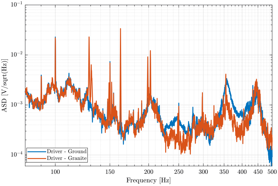
Figure 17: Amplitude Spectral Density of the signal coming from the top geophone (zoom at high frequencies)

3.5 Conclusion

Even tough the Hexapod's driver vibrates quite a lot, it does not generate significant vibrations of the granite when either placed on the granite or on the ground.

Effect on the control system of each stages on the vibration of the station

Table of Contents

1 Effect of all the control systems on the Sample vibrations

1.1 Experimental Setup

1.2 Load data

1.3 Analysis - Time Domain

1.4 Analysis - Frequency Domain

1.4.1 Vibrations at the sample location

1.4.2 Vibrations on the marble

1.5 Conclusion

2 Effect of all the control systems on the Sample vibrations - One stage at a time

2.1 Experimental Setup

2.2 Load data

2.3 Voltage to Velocity

2.4 Analysis - Time Domain

2.5 Analysis - Frequency Domain

2.5.1 Vibrations at the sample location

2.5.2 Vibrations on the marble

2.6 Conclusion

3 Effect of the Symetrie Driver

3.1 Experimental Setup

3.2 Load data

3.3 Analysis - Time Domain

3.4 Analysis - Frequency Domain

3.4.1 Vibrations at the sample location

3.5 Conclusion