Measurements On the Slip-Ring
Table of Contents
- 1. Effect of the Slip-Ring on the signal
- 2. Effect of the rotation of the Slip-Ring
- 3. Measure of the noise induced by the Slip-Ring
- 4. Measure of the noise induced by the slip ring when using a geophone
1 Effect of the Slip-Ring on the signal
The data and matlab files are accessible here.
1.1 Experimental Setup
Two measurements are made with the control systems of all the stages turned OFF.
One geophone is located on the marble while the other is located at the sample location (figure 1).
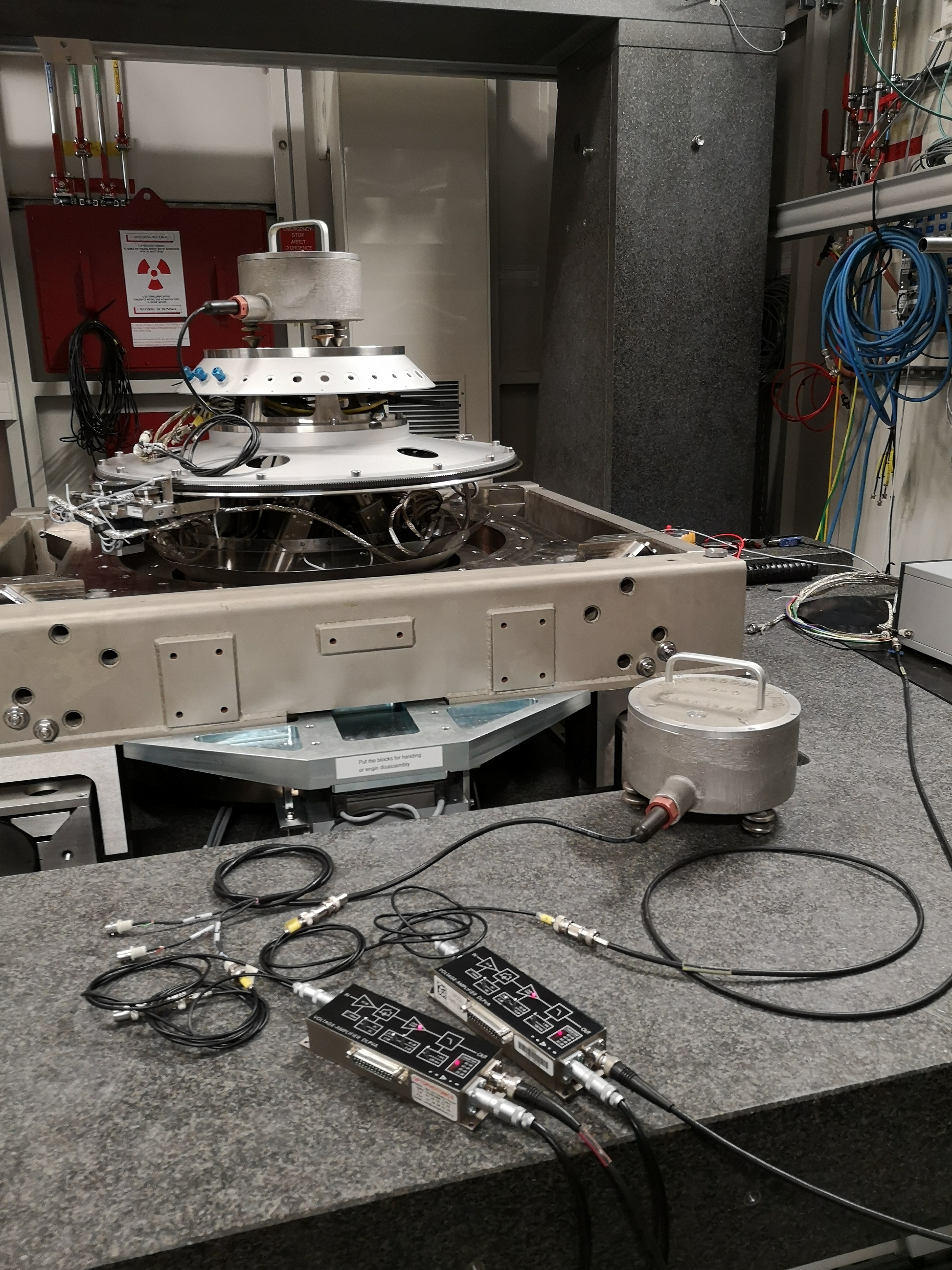
Figure 1: Experimental Setup
The two measurements are:
| Measurement File | Description |
|---|---|
meas_018.mat |
Signal from the top geophone does not goes through the Slip-ring |
meas_019.mat |
Signal goes through the Slip-ring (as shown on the figure above) |
Each of the measurement mat file contains one data array with 3 columns:
| Column number | Description |
|---|---|
| 1 | Geophone - Marble |
| 2 | Geophone - Sample |
| 3 | Time |
1.2 Load data
We load the data of the z axis of two geophones.
d8 = load('mat/data_018.mat', 'data'); d8 = d8.data;
d9 = load('mat/data_019.mat', 'data'); d9 = d9.data;
1.3 Analysis - Time Domain
First, we compare the time domain signals for the two experiments (figure 2).
figure;
hold on;
plot(d9(:, 3), d9(:, 2), 'DisplayName', 'Slip-Ring');
plot(d8(:, 3), d8(:, 2), 'DisplayName', 'Wire');
hold off;
xlabel('Time [s]'); ylabel('Voltage [V]');
xlim([0, 50]);
legend('location', 'northeast');
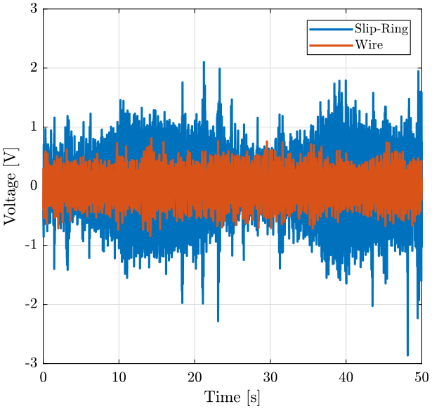
Figure 2: Effect of the Slip-Ring on the measured signal - Time domain
1.4 Analysis - Frequency Domain
We then compute the Power Spectral Density of the two signals and we compare them (figure 3).
dt = d8(2, 3) - d8(1, 3);
Fs = 1/dt;

win = hanning(ceil(1*Fs));
[pxx8, f] = pwelch(d8(:, 2), win, [], [], Fs);
[pxx9, ~] = pwelch(d9(:, 2), win, [], [], Fs);
figure;
hold on;
plot(f, sqrt(pxx9), 'DisplayName', 'Slip-Ring');
plot(f, sqrt(pxx8), 'DisplayName', 'Wire');
hold off;
set(gca, 'xscale', 'log');
set(gca, 'yscale', 'log');
xlabel('Frequency [Hz]'); ylabel('Amplitude Spectral Density $\left[\frac{V}{\sqrt{Hz}}\right]$')
xlim([1, 500]);
legend('Location', 'southwest');
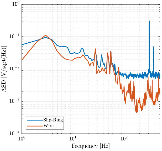
Figure 3: Effect of the Slip-Ring on the measured signal - Frequency domain
1.5 Conclusion
- Connecting the geophone through the Slip-Ring seems to induce a lot of noise.
Remaining questions to answer:
- Why is there a sharp peak at 300Hz?
- Why the use of the Slip-Ring does induce a noise?
- Can the capacitive/inductive properties of the wires in the Slip-ring does not play well with the geophone? (resonant RLC circuit)
2 Effect of the rotation of the Slip-Ring
The data and matlab files are accessible here.
2.1 Measurement Description
Random Signal is generated by one DAC of the SpeedGoat.
The signal going out of the DAC is split into two:
- one BNC cable is directly connected to one ADC of the SpeedGoat
- one BNC cable goes two times in the Slip-Ring (from bottom to top and then from top to bottom) and then is connected to one ADC of the SpeedGoat
Two measurements are done.
| Data File | Description |
|---|---|
mat/data_001.mat |
Slip-ring not turning |
mat/data_002.mat |
Slip-ring turning |
For each measurement, the measured signals are:
| Data File | Description |
|---|---|
t |
Time vector |
x1 |
Direct signal |
x2 |
Signal going through the Slip-Ring |
The goal is to determine is the signal is altered when the spindle is rotating.
Here, the rotation speed of the Slip-Ring is set to 1rpm.
2.2 Load data
We load the data of the z axis of two geophones.
sr_off = load('mat/data_001.mat', 't', 'x1', 'x2');
sr_on  = load('mat/data_002.mat', 't', 'x1', 'x2');
2.3 Analysis
Let's first look at the signal produced by the DAC (figure 4).
figure;
hold on;
plot(sr_on.t,  sr_on.x1);
hold off;
xlabel('Time [s]'); ylabel('Voltage [V]');
xlim([0 10]);
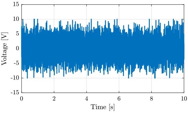
Figure 4: Random signal produced by the DAC
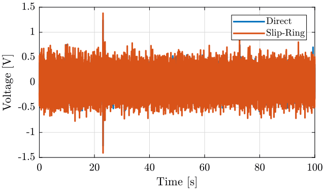
We now look at the difference between the signal directly measured by the ADC and the signal that goes through the slip-ring (figure 5).
figure;
hold on;
plot(sr_on.t,  sr_on.x1  -  sr_on.x2,  'DisplayName', 'Slip-Ring - $\omega = 1rpm$');
plot(sr_off.t, sr_off.x1 - sr_off.x2,'DisplayName', 'Slip-Ring off');
hold off;
xlabel('Time [s]'); ylabel('Voltage [V]');
xlim([0 10]);
legend('Location', 'northeast');
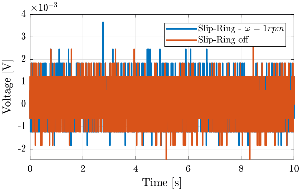
Figure 5: Alteration of the signal when the slip-ring is turning
dt = sr_on.t(2) - sr_on.t(1);
Fs = 1/dt; % [Hz]

win = hanning(ceil(1*Fs));
[pxx_on,  f] = pwelch(sr_on.x1  - sr_on.x2,  win, [], [], Fs);
[pxx_off, ~] = pwelch(sr_off.x1 - sr_off.x2, win, [], [], Fs);
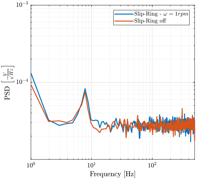
Figure 6: ASD of the measured noise
2.4 Conclusion
Remaining questions:
- Should the measurement be redone using voltage amplifiers?
- Use higher rotation speed and measure for longer periods (to have multiple revolutions) ?
3 Measure of the noise induced by the Slip-Ring
The data and matlab files are accessible here.
3.1 Measurement Description
Goal:
- Determine the noise induced by the slip-ring
Setup:
- 0V is generated by the DAC of the Speedgoat
- Using a T, one part goes directly to the ADC
- The other part goes to the slip-ring 2 times and then to the ADC
- The parameters of the Voltage Amplifier are: 80dB, AC, 1kHz
- Every stage of the station is OFF
First column: Direct measure Second column: Slip-ring measure
Measurements:
data_008: Slip-Ring OFFdata_009: Slip-Ring ONdata_010: Slip-Ring ON and omega=6rpmdata_011: Slip-Ring ON and omega=60rpm
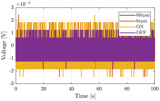
Figure 7: Slip-Ring rotating at 6rpm
Figure 8: Slip-Ring rotating at 60rpm
3.2 Load data
We load the data of the z axis of two geophones.
sr_off = load('mat/data_008.mat', 'data'); sr_off = sr_off.data;
sr_on  = load('mat/data_009.mat', 'data'); sr_on  = sr_on.data;
sr_6r  = load('mat/data_010.mat', 'data'); sr_6r  = sr_6r.data;
sr_60r = load('mat/data_011.mat', 'data'); sr_60r = sr_60r.data;
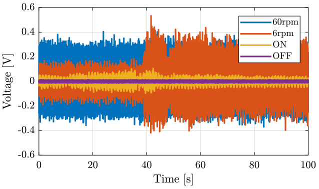
3.3 Time Domain
3.4 Frequency Domain
We first compute some parameters that will be used for the PSD computation.
dt = sr_off(2, 3)-sr_off(1, 3);

Fs = 1/dt; % [Hz]

win = hanning(ceil(10*Fs));
Then we compute the Power Spectral Density using pwelch function.
[pxdir, f] = pwelch(sr_off(:, 1), win, [], [], Fs);
[pxoff, ~] = pwelch(sr_off(:, 2), win, [], [], Fs);
[pxon,  ~] = pwelch(sr_on(:, 2),  win, [], [], Fs);
[px6r,  ~] = pwelch(sr_6r(:, 2),  win, [], [], Fs);
[px60r, ~] = pwelch(sr_60r(:, 2), win, [], [], Fs);
And we plot the ASD of the measured signals (figure 11);
figure;
hold on;
plot(f, sqrt(pxoff), 'DisplayName', 'OFF');
plot(f, sqrt(pxon),  'DisplayName', 'ON');
plot(f, sqrt(px6r),  'DisplayName', '6rpm');
plot(f, sqrt(px60r), 'DisplayName', '60rpm');
plot(f, sqrt(pxdir), 'k-', 'DisplayName', 'Direct');
hold off;
set(gca, 'xscale', 'log');
set(gca, 'yscale', 'log');
xlabel('Frequency [Hz]'); ylabel('ASD of the measured Voltage $\left[\frac{V}{\sqrt{Hz}}\right]$')
legend('Location', 'northeast');
xlim([0.1, 500]);
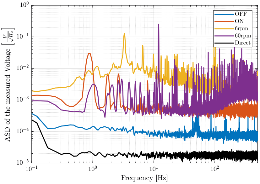
Figure 11: Comparison of the ASD of the measured signals when the slip-ring is ON, OFF and turning
3.5 Conclusion
Questions:
- Why is there some sharp peaks? Can this be due to aliasing?
- It is possible that the amplifiers were saturating during the measurements => should redo the measurements with a low pass filter before the voltage amplifier
4 Measure of the noise induced by the slip ring when using a geophone
The data and matlab files are accessible here.
4.1 First Measurement without LPF
4.1.1 Measurement Description
Goal:
- Determine if the noise induced by the slip-ring is a limiting factor when measuring the signal coming from a geophone
Setup:
- The geophone is located at the sample location
- The two Voltage amplifiers have the same following settings:
- AC
- 60dB
- 1kHz
- The signal from the geophone is split into two using a T-BNC:
- One part goes directly to the voltage amplifier and then to the ADC.
- The other part goes to the slip-ring=>voltage amplifier=>ADC.
First column: Direct measure Second column: Slip-ring measure
Measurements:
data_012: Slip-Ring OFFdata_013: Slip-Ring ON
4.1.2 Load data
We load the data of the z axis of two geophones.
sr_off = load('mat/data_012.mat', 'data'); sr_off = sr_off.data;
sr_on  = load('mat/data_013.mat', 'data'); sr_on  = sr_on.data;
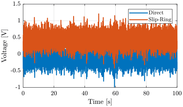
4.1.3 Time Domain
4.1.4 Frequency Domain
We first compute some parameters that will be used for the PSD computation.
dt = sr_off(2, 3)-sr_off(1, 3);

Fs = 1/dt; % [Hz]

win = hanning(ceil(10*Fs));
Then we compute the Power Spectral Density using pwelch function.
% Direct measure
[pxdoff, ~] = pwelch(sr_off(:, 1), win, [], [], Fs);
[pxdon,  ~] = pwelch(sr_on(:, 1),  win, [], [], Fs);

% Slip-Ring measure
[pxsroff, f] = pwelch(sr_off(:, 2), win, [], [], Fs);
[pxsron,  ~] = pwelch(sr_on(:, 2),  win, [], [], Fs);
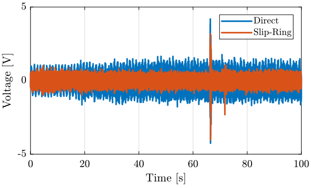
Finally, we compare the Amplitude Spectral Density of the signals (figure 14);
figure;
hold on;
plot(f, sqrt(pxdoff), 'DisplayName', 'Direct - OFF');
plot(f, sqrt(pxsroff), 'DisplayName', 'Slip-Ring - OFF');
plot(f, sqrt(pxdon),  'DisplayName', 'Direct - ON');
plot(f, sqrt(pxsron),  'DisplayName', 'Slip-Ring - ON');
hold off;
set(gca, 'xscale', 'log');
set(gca, 'yscale', 'log');
xlabel('Frequency [Hz]'); ylabel('ASD of the measured Voltage $\left[\frac{V}{\sqrt{Hz}}\right]$')
legend('Location', 'northeast');
xlim([0.1, 500]);
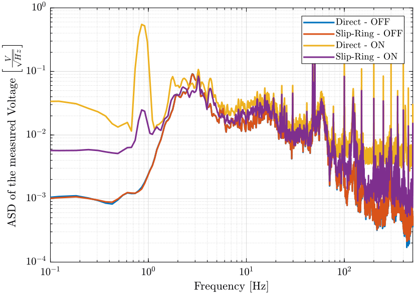
Figure 14: Comparison of the Amplitude Spectral Sensity
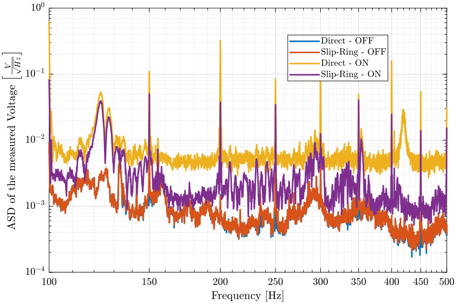
Figure 15: Comparison of the Amplitude Spectral Sensity - Zoom
4.1.5 Conclusion
- The fact that the Slip-Ring is turned ON adds some noise to the signal.
- The signal going through the Slip-Ring is less noisy than the one going directly to the ADC.
- This could be due to less good electromagnetic isolation.
Questions:
- Can the sharp peak on figure 15 be due to the Aliasing?
4.2 Measurement using an oscilloscope
4.2.1 Measurement Setup
Know we are measuring the same signals but using an oscilloscope instead of the Speedgoat ADC.
4.2.2 Observations
Then the Slip-Ring is ON (figure 16), we observe a signal at 40kHz with a peak-to-peak amplitude of 200mV for the direct measure and 100mV for the signal going through the Slip-Ring.
Then the Slip-Ring is OFF, we don't observe this 40kHz anymore (figure 17).
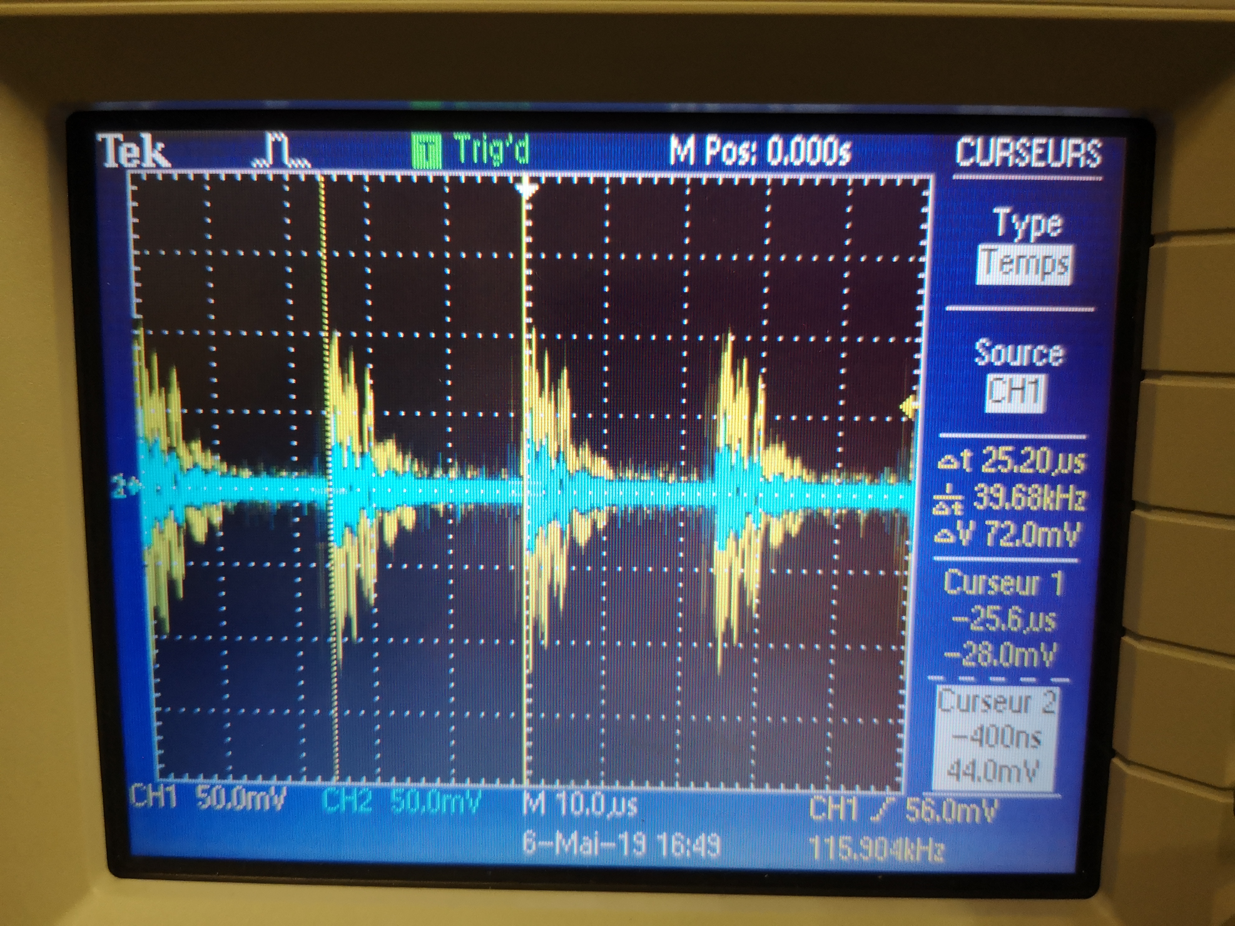
Figure 16: Signals measured by the oscilloscope - Slip-Ring ON - Yellow: Direct measure - Blue: Through Slip-Ring
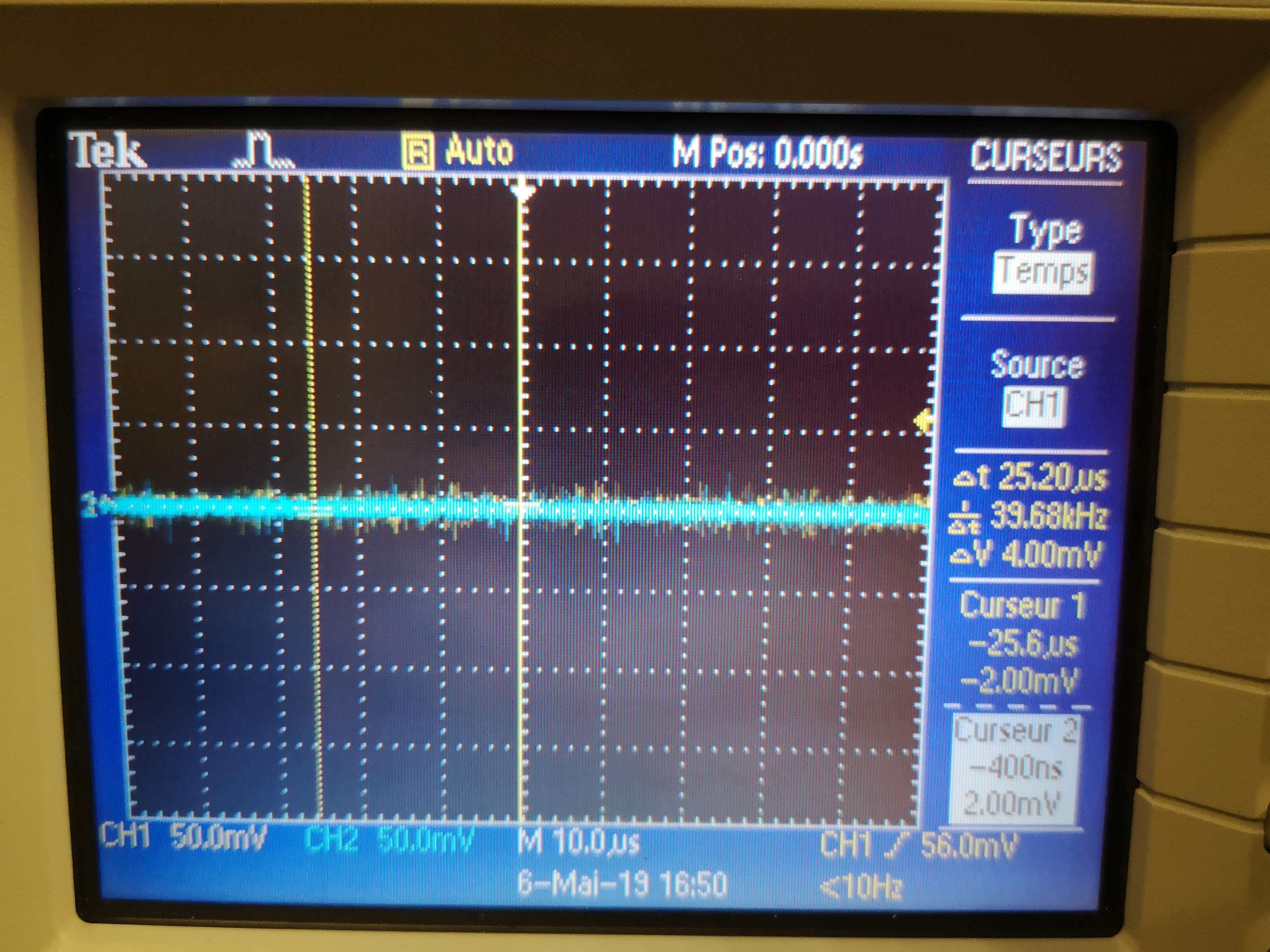
Figure 17: Signals measured by the oscilloscope - Slip-Ring OFF - Yellow: Direct measure - Blue: Through Slip-Ring
4.2.3 Conclusion
- By looking at the signals using an oscilloscope, there is a lot of high frequency noise when turning on the Slip-Ring
- This can eventually saturate the voltage amplifiers (seen by a led indicating saturation)
- The choice is to add a Low pass filter before the voltage amplifiers to not saturate them and filter the noise.
4.3 New measurements with a LPF before the Voltage Amplifiers
4.3.1 Setup description
A first order low pass filter is added before the Voltage Amplifiers with the following values:
\begin{aligned} R &= 1k\Omega \\ C &= 1\mu F \end{aligned}And we have a cut-off frequency of \(f_c = \frac{1}{RC} = 160Hz\).
We are measuring the signal from a geophone put on the marble with and without the added LPF:
- with the slip ring OFF:
mat/data_016.mat - with the slip ring ON:
mat/data_017.mat
4.3.2 Load data
We load the data of the z axis of two geophones.
sr_lpf_off = load('mat/data_016.mat', 'data'); sr_lpf_off = sr_lpf_off.data;
sr_lpf_on  = load('mat/data_017.mat', 'data'); sr_lpf_on  = sr_lpf_on.data;
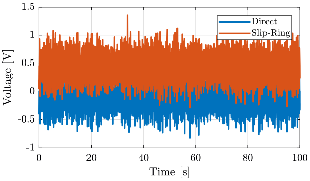
4.3.3 Time Domain
4.3.4 Frequency Domain
We first compute some parameters that will be used for the PSD computation.
dt = sr_lpf_off(2, 3)-sr_lpf_off(1, 3);

Fs = 1/dt; % [Hz]

win = hanning(ceil(10*Fs));
Then we compute the Power Spectral Density using pwelch function.
% Direct measure
[pxd_lpf_off, ~] = pwelch(sr_lpf_off(:, 1), win, [], [], Fs);
[pxd_lpf_on,  ~] = pwelch(sr_lpf_on(:, 1),  win, [], [], Fs);

% Slip-Ring measure
[pxsr_lpf_off, f] = pwelch(sr_lpf_off(:, 2), win, [], [], Fs);
[pxsr_lpf_on,  ~] = pwelch(sr_lpf_on(:, 2),  win, [], [], Fs);
Finally, we compare the Amplitude Spectral Density of the signals (figure 20);
figure;
hold on;
plot(f, sqrt(pxd_lpf_off), 'DisplayName', 'Direct - OFF');
plot(f, sqrt(pxsr_lpf_off), 'DisplayName', 'Slip-Ring - OFF');
plot(f, sqrt(pxd_lpf_on),  'DisplayName', 'Direct - ON');
plot(f, sqrt(pxsr_lpf_on),  'DisplayName', 'Slip-Ring - ON');
hold off;
set(gca, 'xscale', 'log');
set(gca, 'yscale', 'log');
xlabel('Frequency [Hz]'); ylabel('ASD of the measured Voltage $\left[\frac{V}{\sqrt{Hz}}\right]$')
legend('Location', 'northeast');
xlim([0.1, 500]);
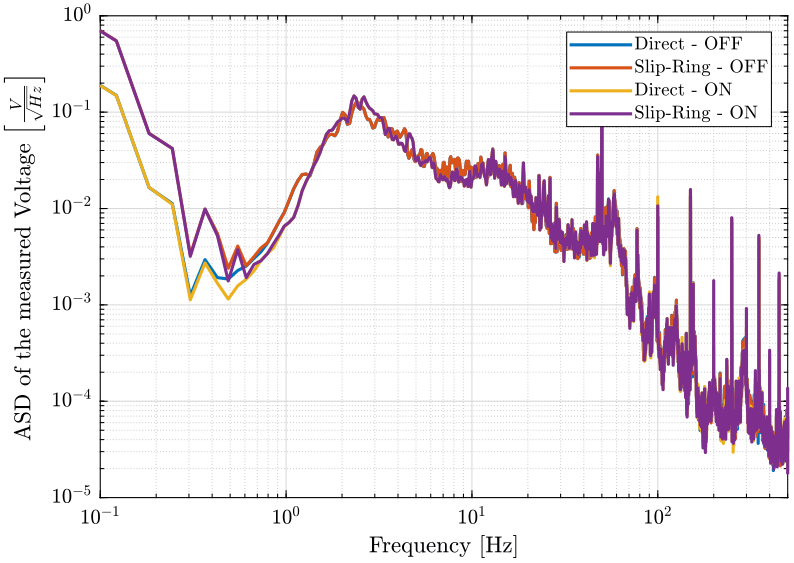
Figure 20: Comparison of the Amplitude Spectral Sensity
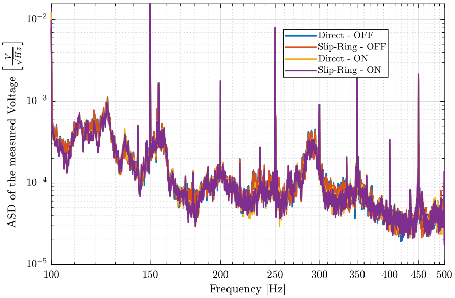
Figure 21: Comparison of the Amplitude Spectral Sensity - Zoom
4.3.5 Comparison of with and without LPF
figure;
hold on;
plot(f, sqrt(pxdon),  'DisplayName', 'Direct - ON');
plot(f, sqrt(pxsron),  'DisplayName', 'Slip-Ring - ON');
plot(f, sqrt(pxd_lpf_on),  'DisplayName', 'Direct - ON - LPF');
plot(f, sqrt(pxsr_lpf_on),  'DisplayName', 'Slip-Ring - ON - LPF');
hold off;
set(gca, 'xscale', 'log');
set(gca, 'yscale', 'log');
xlabel('Frequency [Hz]'); ylabel('ASD of the measured Voltage $\left[\frac{V}{\sqrt{Hz}}\right]$')
legend('Location', 'northeast');
xlim([0.1, 500]);
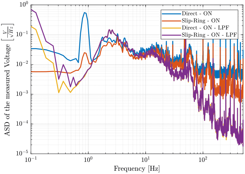
Figure 22: Comparison of the measured signals with and without LPF
4.3.6 Conclusion
- Using the LPF, we don't have any perturbation coming from the slip-ring when it is on.
- However, we should use a smaller value of the capacitor to have a cut-off frequency at \(1kHz\).