Huddle Test of the L22 Geophones
Table of Contents
- 1. Experimental Setup
- 2. Signal Processing
- 2.1. Load data
- 2.2. Time Domain Data
- 2.3. Computation of the ASD of the measured voltage
- 2.4. Scaling to take into account the sensibility of the geophone and the voltage amplifier
- 2.5. Computation of the ASD of the velocity
- 2.6. Transfer function between the two geophones
- 2.7. Estimation of the sensor noise
- 3. Compare axis
- 4. Appendix
1 Experimental Setup
Two L22 geophones are used. They are placed on the ID31 granite. They are leveled.
The signals are amplified using voltage amplifier with a gain of 60dB. The voltage amplifiers include a low pass filter with a cut-off frequency at 1kHz.
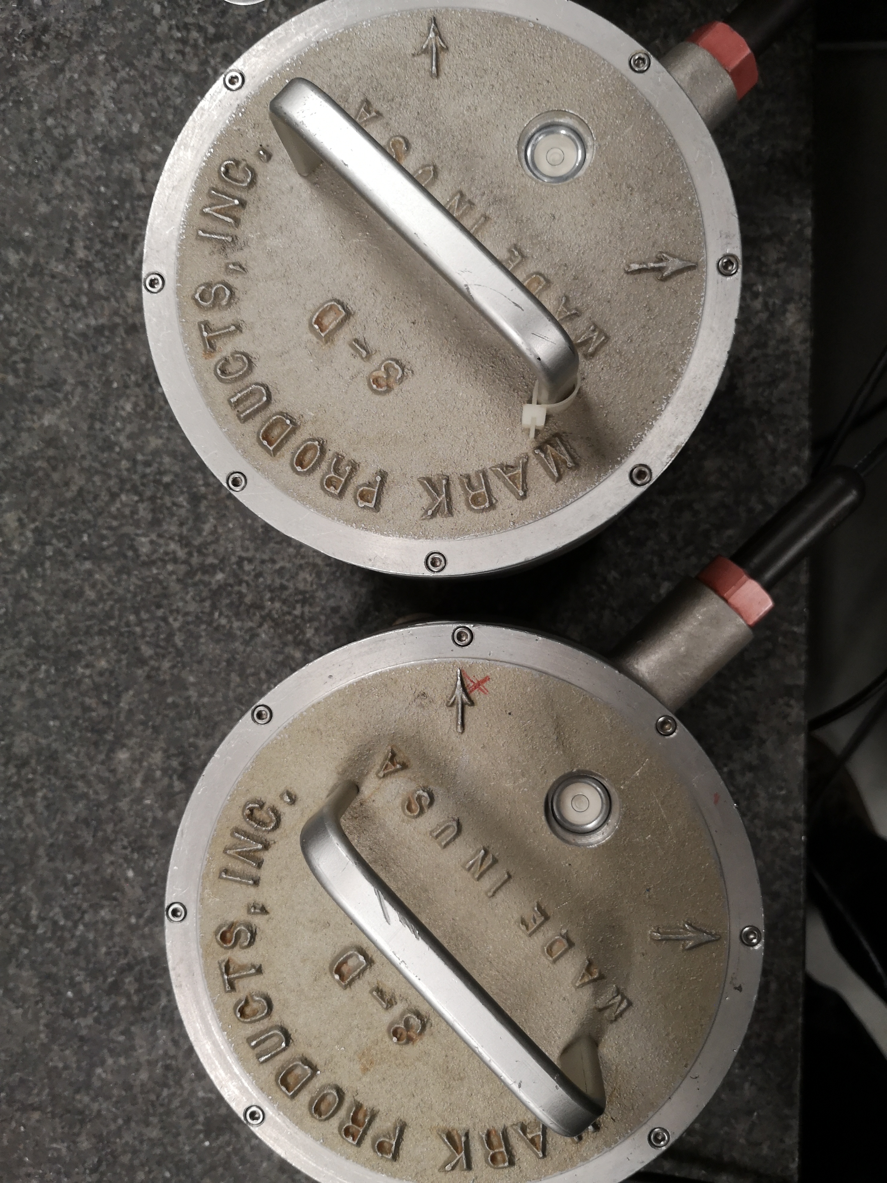
Figure 1: Setup
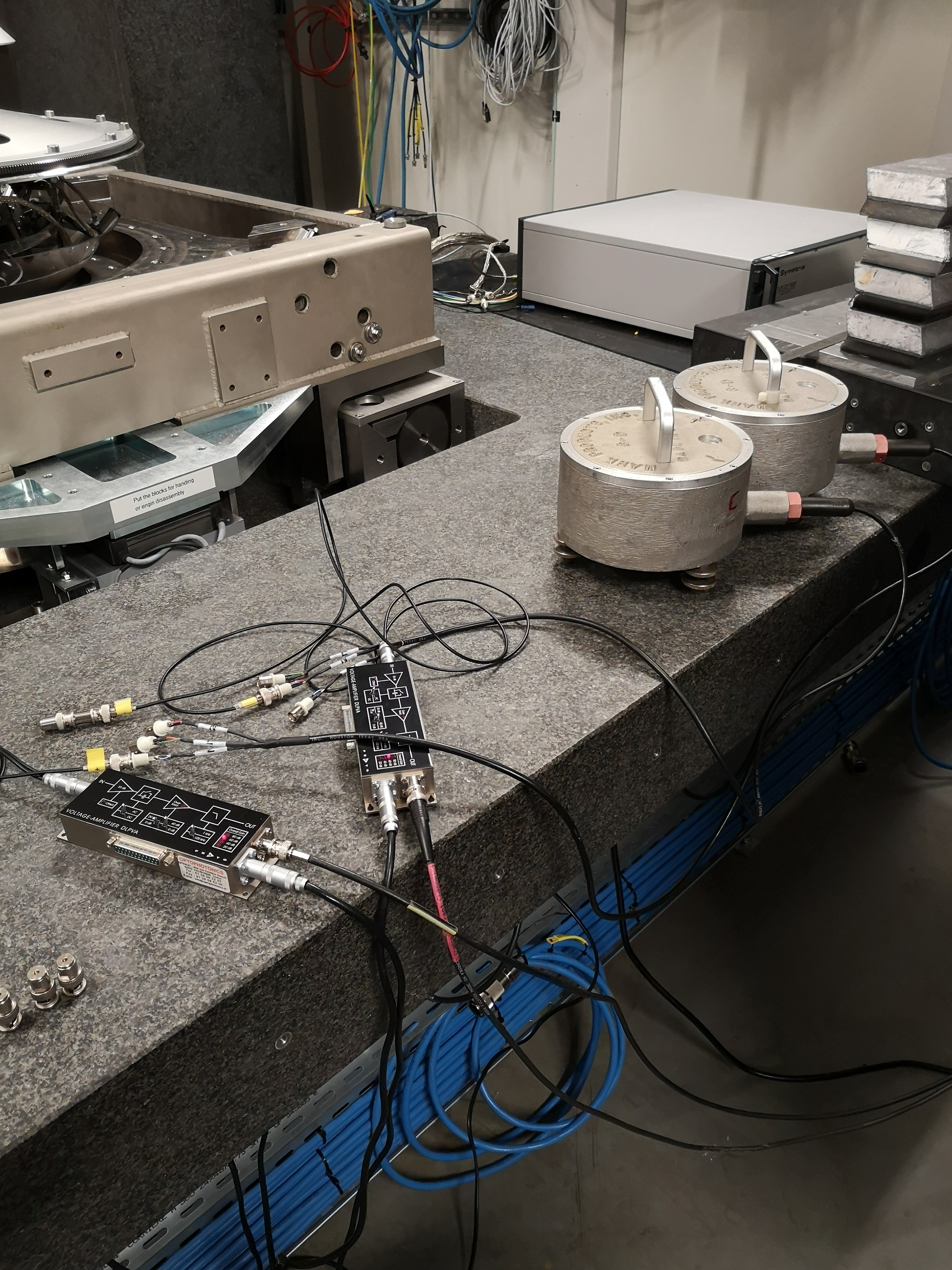
Figure 2: Geophones
2 Signal Processing
The Matlab computing file for this part is accessible here.
The mat file containing the measurement data is accessible here.
2.1 Load data
We load the data of the z axis of two geophones.
load('mat/data_001.mat', 't', 'x1', 'x2');
dt = t(2) - t(1);
2.2 Time Domain Data
figure;
hold on;
plot(t, x1);
plot(t, x2);
hold off;
xlabel('Time [s]');
ylabel('Voltage [V]');
xlim([t(1), t(end)]);
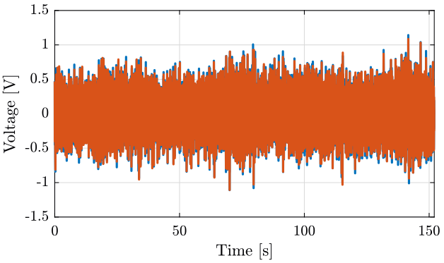
Figure 3: Time domain Data
figure;
hold on;
plot(t, x1);
plot(t, x2);
hold off;
xlabel('Time [s]');
ylabel('Voltage [V]');
xlim([0 1]);
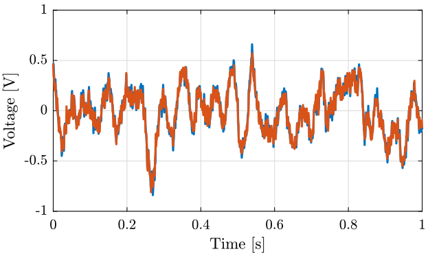
Figure 4: Time domain Data - Zoom
2.3 Computation of the ASD of the measured voltage
We first define the parameters for the frequency domain analysis.
win = hanning(ceil(length(x1)/100));
Fs = 1/dt;
[pxx1, f] = pwelch(x1, win, [], [], Fs);
[pxx2, ~] = pwelch(x2, win, [], [], Fs);
2.4 Scaling to take into account the sensibility of the geophone and the voltage amplifier
The Geophone used are L22. Their sensibility are shown on figure 5.
S0 = 88; % Sensitivity [V/(m/s)]
f0 = 2; % Cut-off frequnecy [Hz]
S = (s/2/pi/f0)/(1+s/2/pi/f0);
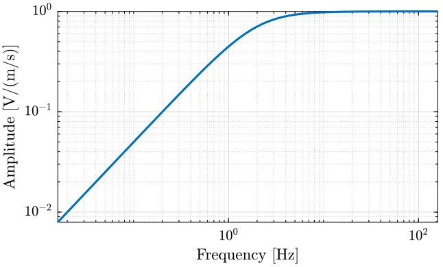
Figure 5: Sensibility of the Geophone
We also take into account the gain of the electronics which is here set to be \(60dB\). The amplifiers also include a low pass filter with a cut-off frequency set at 1kHz.
G0 = 60; % [dB]

G = 10^(G0/20)/(1+s/2/pi/1000);
We divide the ASD measured (in \(\text{V}/\sqrt{\text{Hz}}\)) by the transfer function of the voltage amplifier to obtain the ASD of the voltage across the geophone. We further divide the result by the sensibility of the Geophone to obtain the ASD of the velocity in \(m/s/\sqrt{Hz}\).
scaling = 1./squeeze(abs(freqresp(G*S, f, 'Hz')));
2.5 Computation of the ASD of the velocity
The ASD of the measured velocity is shown on figure 6.
figure;
hold on;
plot(f, sqrt(pxx1).*scaling);
plot(f, sqrt(pxx2).*scaling);
hold off;
set(gca, 'xscale', 'log');
set(gca, 'yscale', 'log');
xlabel('Frequency [Hz]'); ylabel('PSD [m/s/sqrt(Hz)]')
xlim([2, 500]);
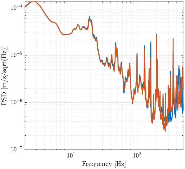
Figure 6: Spectral density of the velocity
We also plot the ASD in displacement (figure 7);
figure;
hold on;
plot(f, (pxx1.*scaling./f).^2);
plot(f, (pxx2.*scaling./f).^2);
hold off;
set(gca, 'xscale', 'log'); set(gca, 'yscale', 'log');
xlabel('Frequency [Hz]'); ylabel('PSD [m/s/sqrt(Hz)]')
xlim([2, 500]);
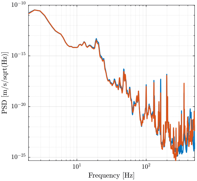
Figure 7: Amplitude Spectral Density of the displacement as measured by the geophones
2.6 Transfer function between the two geophones
We here compute the transfer function from one geophone to the other. The result is shown on figure 8.
We also compute the coherence between the two signals (figure 9).
[T12, ~] = tfestimate(x1, x2, win, [], [], Fs);
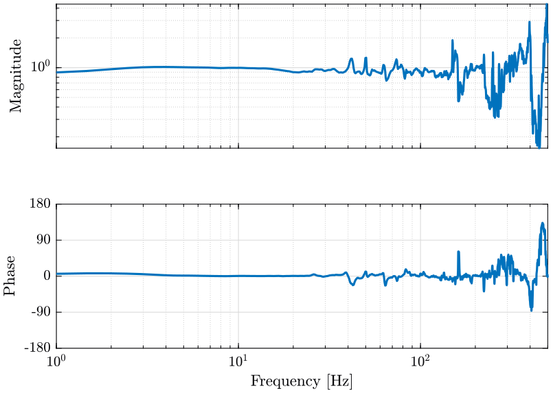
Figure 8: Estimated transfer function between the two geophones
[coh12, ~] = mscohere(x1, x2, win, [], [], Fs);
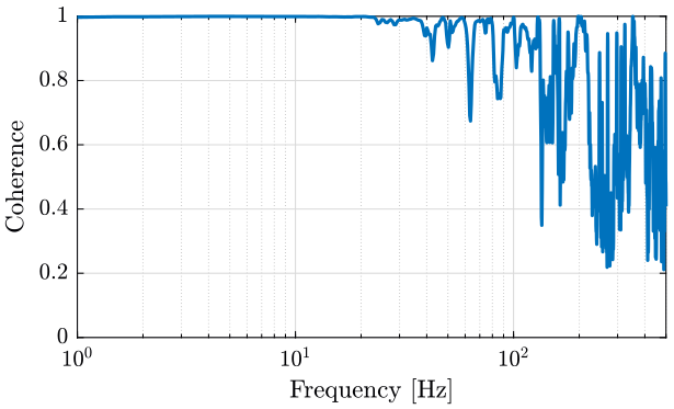
Figure 9: Cohererence between the signals of the two geophones
2.7 Estimation of the sensor noise
The technique to estimate the sensor noise is taken from barzilai98_techn_measur_noise_sensor_presen.
The coherence between signals \(X\) and \(Y\) is defined as follow \[ \gamma^2_{XY}(\omega) = \frac{|G_{XY}(\omega)|^2}{|G_{X}(\omega)| |G_{Y}(\omega)|} \] where \(|G_X(\omega)|\) is the output Power Spectral Density (PSD) of signal \(X\) and \(|G_{XY}(\omega)|\) is the Cross Spectral Density (CSD) of signal \(X\) and \(Y\).
The PSD and CSD are defined as follow:
\begin{align} |G_X(\omega)| &= \frac{2}{n_d T} \sum^{n_d}_{n=1} \left| X_k(\omega, T) \right|^2 \\ |G_{XY}(\omega)| &= \frac{2}{n_d T} \sum^{n_d}_{n=1} [ X_k^*(\omega, T) ] [ Y_k(\omega, T) ] \end{align}where:
- \(n_d\) is the number for records averaged
- \(T\) is the length of each record
- \(X_k(\omega, T)\) is the finite Fourier transform of the kth record
- \(X_k^*(\omega, T)\) is its complex conjugate
The mscohere function is compared with this formula on Appendix (section 4.1), it is shown that it is identical.
Figure 10 illustrate a block diagram model of the system used to determine the sensor noise of the geophone.
Two geophones are mounted side by side to ensure that they are exposed by the same motion input \(U\).
Each sensor has noise \(N\) and \(M\).
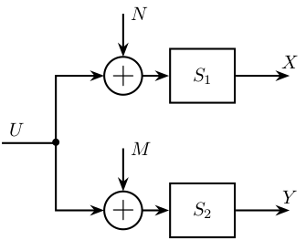
Figure 10: Huddle test block diagram
We here assume that each sensor has the same magnitude of instrumental noise (\(N = M\)). We also assume that \(S_1 = S_2 = 1\).
We then obtain:
\begin{equation} \label{org5b2976f} \gamma_{XY}^2(\omega) = \frac{1}{1 + 2 \left( \frac{|G_N(\omega)|}{|G_U(\omega)|} \right) + \left( \frac{|G_N(\omega)|}{|G_U(\omega)|} \right)^2} \end{equation}Since the input signal \(U\) and the instrumental noise \(N\) are incoherent:
\begin{equation} \label{orgb493a2c} |G_X(\omega)| = |G_N(\omega)| + |G_U(\omega)| \end{equation}From equations \eqref{org5b2976f} and \eqref{orgb493a2c}, we finally obtain
The instrumental noise is computed below. The result in V2/Hz is shown on figure 11.
pxxN = pxx1.*(1 - coh12);
figure;
hold on;
plot(f, pxx1, '-');
plot(f, pxx2, '-');
plot(f, pxxN, 'k--');
hold off;
set(gca, 'xscale', 'log'); set(gca, 'yscale', 'log');
xlabel('Frequency [Hz]'); ylabel('PSD [$V^2/Hz$]');
xlim([1, 500]);
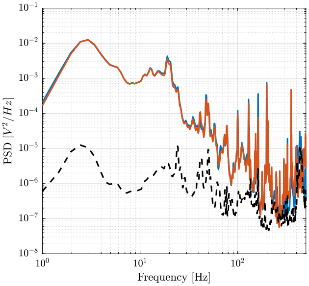
Figure 11: Instrumental Noise and Measurement in \(V^2/Hz\)
This is then further converted into velocity and compared with the ground velocity measurement. (figure 12)
figure;
hold on;
plot(f, sqrt(pxx1).*scaling, '-');
plot(f, sqrt(pxx2).*scaling, '-');
plot(f, sqrt(pxxN).*scaling, 'k--');
hold off;
set(gca, 'xscale', 'log'); set(gca, 'yscale', 'log');
xlabel('Frequency [Hz]'); ylabel('PSD [$m/s/\sqrt{Hz}$]');
xlim([1, 500]);
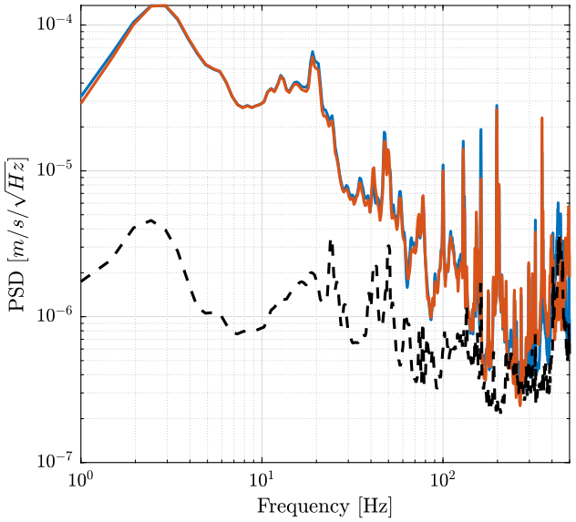
Figure 12: Instrumental Noise and Measurement in \(m/s/\sqrt{Hz}\)
3 Compare axis
The Matlab computing file for this part is accessible here.
The mat files containing the measurement data are accessible with the following links:
3.1 Load data
We first load the data for the three axis.
z     = load('mat/data_001.mat', 't', 'x1', 'x2');
east  = load('mat/data_002.mat', 't', 'x1', 'x2');
north = load('mat/data_003.mat', 't', 'x1', 'x2');
3.2 Compare PSD
The PSD for each axis of the two geophones are computed.
[pz1, fz] = pwelch(z.x1, hanning(ceil(length(z.x1)/100)), [], [], 1/(z.t(2)-z.t(1)));
[pz2, ~]  = pwelch(z.x2, hanning(ceil(length(z.x2)/100)), [], [], 1/(z.t(2)-z.t(1)));

[pe1, fe] = pwelch(east.x1, hanning(ceil(length(east.x1)/100)), [], [], 1/(east.t(2)-east.t(1)));
[pe2, ~]  = pwelch(east.x2, hanning(ceil(length(east.x2)/100)), [], [], 1/(east.t(2)-east.t(1)));

[pn1, fn] = pwelch(north.x1, hanning(ceil(length(north.x1)/100)), [], [], 1/(north.t(2)-north.t(1)));
[pn2, ~]  = pwelch(north.x2, hanning(ceil(length(north.x2)/100)), [], [], 1/(north.t(2)-north.t(1)));
We compare them. The result is shown on figure 13.
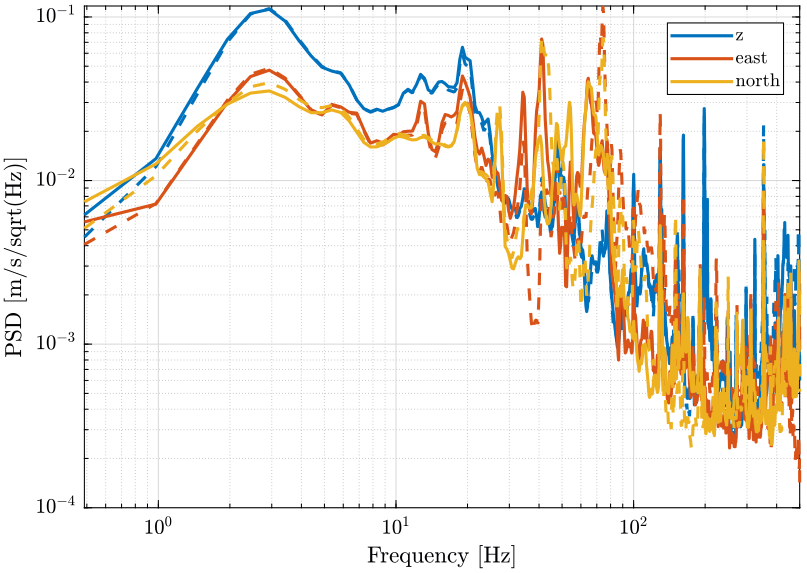
Figure 13: Compare the measure PSD of the two geophones for the three axis
3.3 Compare TF
The transfer functions from one geophone to the other are also computed for each axis. The result is shown on figure 14.
[Tz, fz] = tfestimate(z.x1, z.x2, hanning(ceil(length(z.x1)/100)), [], [], 1/(z.t(2)-z.t(1)));
[Te, fe] = tfestimate(east.x1, east.x2, hanning(ceil(length(east.x1)/100)), [], [], 1/(east.t(2)-east.t(1)));
[Tn, fn] = tfestimate(north.x1, north.x2, hanning(ceil(length(north.x1)/100)), [], [], 1/(north.t(2)-north.t(1)));
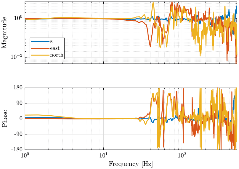
Figure 14: Compare the transfer function from one geophone to the other for the 3 axis
4 Appendix
4.1 Computation of coherence from PSD and CSD
load('mat/data_001.mat', 't', 'x1', 'x2');
dt = t(2) - t(1);
Fs = 1/dt;
win = hanning(ceil(length(x1)/100));
pxy = cpsd(x1, x2, win, [], [], Fs);
pxx = pwelch(x1, win, [], [], Fs);
pyy = pwelch(x2, win, [], [], Fs);
coh = mscohere(x1, x2, win, [], [], Fs);
figure;
hold on;
plot(f, abs(pxy).^2./abs(pxx)./abs(pyy), '-');
plot(f, coh, '--');
hold off;
set(gca, 'xscale', 'log');
xlabel('Frequency'); ylabel('Coherence');
xlim([1, 500]);
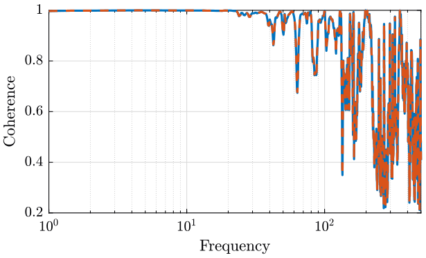
Figure 15: Comparison of mscohere and manual computation
Bibliography
- [barzilai98_techn_measur_noise_sensor_presen] Aaron Barzilai, Tom VanZandt & Tom Kenny, Technique for Measurement of the Noise of a Sensor in the Presence of Large Background Signals, Review of Scientific Instruments, 69(7), 2767-2772 (1998). link. doi.