Measurements

1. Effect of all the control systems on the Sample vibrations
2. Effect of all the control systems on the Sample vibrations - One stage at a time
3. Effect of the Symetrie Driver
4. Transfer function from one stage to the other

For all the measurements shown here:

geophones used are L22 with a resonance frequency of 1Hz
the signals are amplified with voltage amplifiers with a gain of 60dB
the voltage amplifiers include a low pass filter with a cut-off frequency at 1kHz

1 Effect of all the control systems on the Sample vibrations

All the files (data and Matlab scripts) are accessible here.

1.1 Experimental Setup

We here measure the signals of two geophones:

One is located on top of the Sample platform
One is located on the marble

The signal from the top geophone does not go trought the slip-ring.

First, all the control systems are turned ON, then, they are turned one by one. Each measurement are done during 50s.

Table 1: Summary of the measurements and the states of the control systems
Ty	Ry	Slip Ring	Spindle	Hexapod	Meas. file
ON	ON	ON	ON	ON	`meas_003.mat`
OFF	ON	ON	ON	ON	`meas_004.mat`
OFF	OFF	ON	ON	ON	`meas_005.mat`
OFF	OFF	OFF	ON	ON	`meas_006.mat`
OFF	OFF	OFF	OFF	ON	`meas_007.mat`
OFF	OFF	OFF	OFF	OFF	`meas_008.mat`

Each of the mat file contains one array data with 3 columns:

Column number	Description
1	Geophone - Marble
2	Geophone - Sample
3	Time

1.2 Load data

We load the data of the z axis of two geophones.

d3 = load('mat/data_003.mat', 'data'); d3 = d3.data;
d4 = load('mat/data_004.mat', 'data'); d4 = d4.data;
d5 = load('mat/data_005.mat', 'data'); d5 = d5.data;
d6 = load('mat/data_006.mat', 'data'); d6 = d6.data;
d7 = load('mat/data_007.mat', 'data'); d7 = d7.data;
d8 = load('mat/data_008.mat', 'data'); d8 = d8.data;

1.3 Analysis - Time Domain

First, we can look at the time domain data and compare all the measurements:

comparison for the geophone at the sample location (figure 1)
comparison for the geophone on the granite (figure 2)

figure;
hold on;
plot(d3(:, 3), d3(:, 2), 'DisplayName', 'All ON');
plot(d4(:, 3), d4(:, 2), 'DisplayName', 'Ty OFF');
plot(d5(:, 3), d5(:, 2), 'DisplayName', 'Ry OFF');
plot(d6(:, 3), d6(:, 2), 'DisplayName', 'S-R OFF');
plot(d7(:, 3), d7(:, 2), 'DisplayName', 'Rz OFF');
plot(d8(:, 3), d8(:, 2), 'DisplayName', 'Hexa OFF');
hold off;
xlabel('Time [s]'); ylabel('Voltage [V]');
xlim([0, 50]);
legend('Location', 'bestoutside');

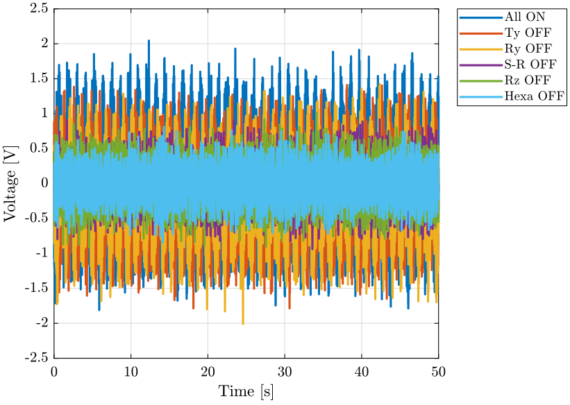
Figure 1: Comparison of the time domain data when turning off the control system of the stages - Geophone at the sample location

figure;
hold on;
plot(d3(:, 3), d3(:, 1), 'DisplayName', 'All ON');
plot(d4(:, 3), d4(:, 1), 'DisplayName', 'Ty OFF');
plot(d5(:, 3), d5(:, 1), 'DisplayName', 'Ry OFF');
plot(d6(:, 3), d6(:, 1), 'DisplayName', 'S-R OFF');
plot(d7(:, 3), d7(:, 1), 'DisplayName', 'Rz OFF');
plot(d8(:, 3), d8(:, 1), 'DisplayName', 'Hexa OFF');
hold off;
xlabel('Time [s]'); ylabel('Voltage [V]');
xlim([0, 50]);
legend('Location', 'bestoutside');

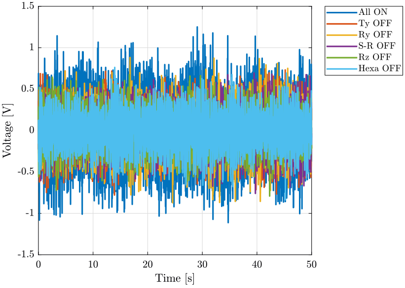
Figure 2: Comparison of the time domain data when turning off the control system of the stages - Geophone on the marble

1.4 Analysis - Frequency Domain

dt = d3(2, 3) - d3(1, 3);

Fs = 1/dt;
win = hanning(ceil(10*Fs));

1.4.1 Vibrations at the sample location

First, we compute the Power Spectral Density of the signals coming from the Geophone located at the sample location.

[px3, f] = pwelch(d3(:, 2), win, [], [], Fs);
[px4, ~] = pwelch(d4(:, 2), win, [], [], Fs);
[px5, ~] = pwelch(d5(:, 2), win, [], [], Fs);
[px6, ~] = pwelch(d6(:, 2), win, [], [], Fs);
[px7, ~] = pwelch(d7(:, 2), win, [], [], Fs);
[px8, ~] = pwelch(d8(:, 2), win, [], [], Fs);

And we compare all the signals (figures 3 and 4).

figure;
hold on;
plot(f, sqrt(px3), 'DisplayName', 'All ON');
plot(f, sqrt(px4), 'DisplayName', 'Ty OFF');
plot(f, sqrt(px5), 'DisplayName', 'Ry OFF');
plot(f, sqrt(px6), 'DisplayName', 'S-R OFF');
plot(f, sqrt(px7), 'DisplayName', 'Rz OFF');
plot(f, sqrt(px8), 'DisplayName', 'Hexa OFF');
hold off;
set(gca, 'xscale', 'log');
set(gca, 'yscale', 'log');
xlabel('Frequency [Hz]'); ylabel('Amplitude Spectral Density $\left[\frac{V}{\sqrt{Hz}}\right]$')
xlim([0.1, 500]);
legend('Location', 'southwest');

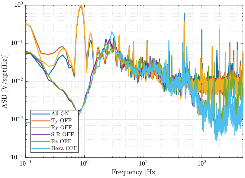
Figure 3: Amplitude Spectral Density of the signal coming from the top geophone

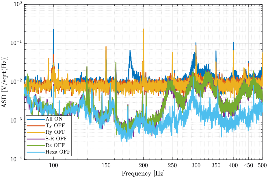
Figure 4: Amplitude Spectral Density of the signal coming from the top geophone (zoom at high frequencies)

1.4.2 Vibrations on the marble

Now we plot the same curves for the geophone located on the marble.

[px3, f] = pwelch(d3(:, 1), win, [], [], Fs);
[px4, ~] = pwelch(d4(:, 1), win, [], [], Fs);
[px5, ~] = pwelch(d5(:, 1), win, [], [], Fs);
[px6, ~] = pwelch(d6(:, 1), win, [], [], Fs);
[px7, ~] = pwelch(d7(:, 1), win, [], [], Fs);
[px8, ~] = pwelch(d8(:, 1), win, [], [], Fs);

And we compare the Amplitude Spectral Densities (figures 5 and 6)

figure;
hold on;
plot(f, sqrt(px3), 'DisplayName', 'All ON');
plot(f, sqrt(px4), 'DisplayName', 'Ty OFF');
plot(f, sqrt(px5), 'DisplayName', 'Ry OFF');
plot(f, sqrt(px6), 'DisplayName', 'S-R OFF');
plot(f, sqrt(px7), 'DisplayName', 'Rz OFF');
plot(f, sqrt(px8), 'DisplayName', 'Hexa OFF');
hold off;
set(gca, 'xscale', 'log');
set(gca, 'yscale', 'log');
xlabel('Frequency [Hz]'); ylabel('Amplitude Spectral Density $\left[\frac{V}{\sqrt{Hz}}\right]$')
xlim([0.1, 500]);
legend('Location', 'northeast');

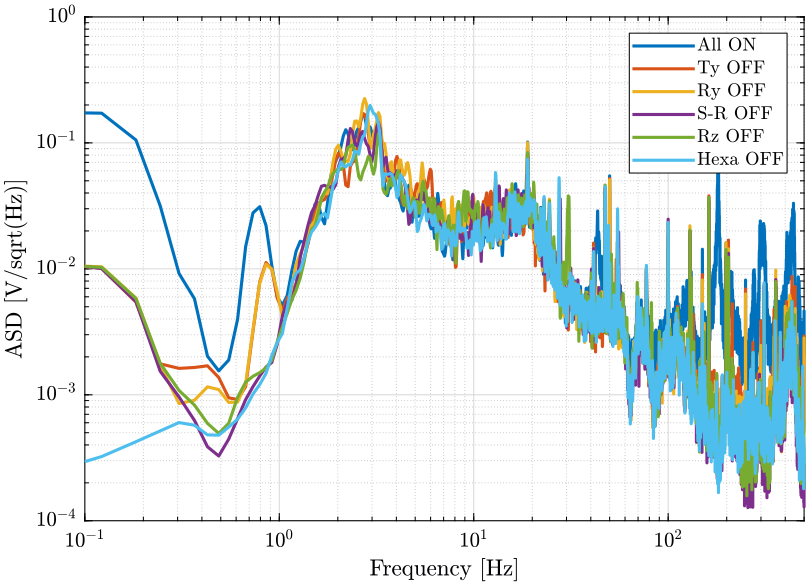
Figure 5: Amplitude Spectral Density of the signal coming from the top geophone

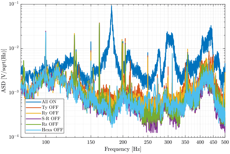
Figure 6: Amplitude Spectral Density of the signal coming from the top geophone (zoom at high frequencies)

1.5 Effect of the control system on the transmissibility from ground to sample

As the feedback loops change the dynamics of the system, we should see differences on the transfer function from marble velocity to sample velocity when turning off the control systems (figure 7).

dt = d3(2, 3) - d3(1, 3);

Fs = 1/dt;
win = hanning(ceil(1*Fs));

First, we compute the Power Spectral Density of the signals coming from the Geophone located at the sample location.

[T3, f] = tfestimate(d3(:, 1), d3(:, 2), win, [], [], Fs);
[T4, ~] = tfestimate(d4(:, 1), d4(:, 2), win, [], [], Fs);
[T5, ~] = tfestimate(d5(:, 1), d5(:, 2), win, [], [], Fs);
[T6, ~] = tfestimate(d6(:, 1), d6(:, 2), win, [], [], Fs);
[T7, ~] = tfestimate(d7(:, 1), d7(:, 2), win, [], [], Fs);
[T8, ~] = tfestimate(d8(:, 1), d8(:, 2), win, [], [], Fs);

figure;
ax1 = subplot(2, 1, 1);
hold on;
plot(f, abs(T3), 'DisplayName', 'All ON');
plot(f, abs(T4), 'DisplayName', 'Ty OFF');
plot(f, abs(T5), 'DisplayName', 'Ry OFF');
plot(f, abs(T6), 'DisplayName', 'S-R OFF');
plot(f, abs(T7), 'DisplayName', 'Rz OFF');
plot(f, abs(T8), 'DisplayName', 'Hexa OFF');
hold off;
set(gca, 'xscale', 'log'); set(gca, 'yscale', 'log');
set(gca, 'XTickLabel',[]);
ylabel('Magnitude');
legend('Location', 'northwest');

ax2 = subplot(2, 1, 2);
hold on;
plot(f, mod(180+180/pi*phase(T3), 360)-180);
plot(f, mod(180+180/pi*phase(T4), 360)-180);
plot(f, mod(180+180/pi*phase(T5), 360)-180);
plot(f, mod(180+180/pi*phase(T6), 360)-180);
plot(f, mod(180+180/pi*phase(T7), 360)-180);
plot(f, mod(180+180/pi*phase(T8), 360)-180);
hold off;
set(gca, 'xscale', 'log');
ylim([-180, 180]);
yticks([-180, -90, 0, 90, 180]);
xlabel('Frequency [Hz]'); ylabel('Phase');

linkaxes([ax1,ax2],'x');
xlim([1, 500]);

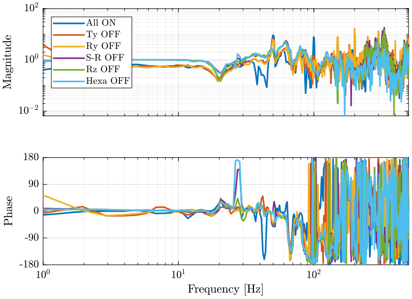
Figure 7: Comparison of the transfer function from the geophone on the marble to the geophone at the sample location

1.6 Conclusion

The control system of the Ty stage induces a lot of vibrations of the marble

Why it seems that the measurement noise at high frequency is the limiting factor when the slip ring is ON but not when it is OFF?

2 Effect of all the control systems on the Sample vibrations - One stage at a time

All the files (data and Matlab scripts) are accessible here.

2.1 Experimental Setup

We here measure the signals of two geophones:

One is located on top of the Sample platform
One is located on the marble

The signal from the top geophone does go trought the slip-ring.

All the control systems are turned OFF, then, they are turned on one at a time.

Each measurement are done during 100s.

The settings of the voltage amplifier are shown on figure 8. A first order low pass filter with a cut-off frequency of 1kHz is added before the voltage amplifier.

Table 2: Summary of the measurements and the states of the control systems
Ty	Ry	Slip Ring	Spindle	Hexapod	Meas. file
OFF	OFF	OFF	OFF	OFF	`meas_013.mat`
ON	OFF	OFF	OFF	OFF	`meas_014.mat`
OFF	ON	OFF	OFF	OFF	`meas_015.mat`
OFF	OFF	ON	OFF	OFF	`meas_016.mat`
OFF	OFF	OFF	ON	OFF	`meas_017.mat`
OFF	OFF	OFF	OFF	ON	`meas_018.mat`

Each of the mat file contains one array data with 3 columns:

Column number	Description
1	Geophone - Marble
2	Geophone - Sample
3	Time

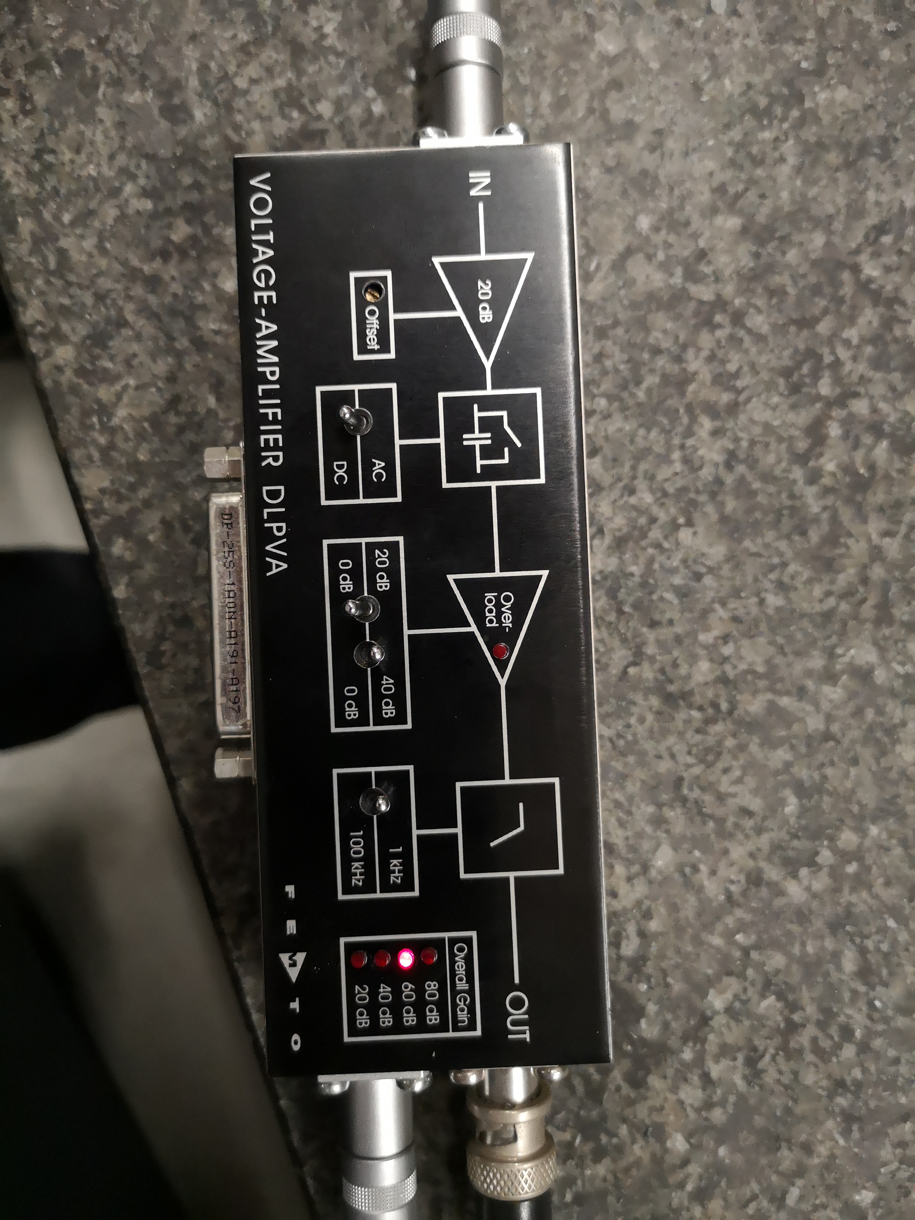
Figure 8: Voltage amplifier settings for the measurement

2.2 Load data

We load the data of the z axis of two geophones.

d_of = load('mat/data_013.mat', 'data'); d_of = d_of.data;
d_ty = load('mat/data_014.mat', 'data'); d_ty = d_ty.data;
d_ry = load('mat/data_015.mat', 'data'); d_ry = d_ry.data;
d_sr = load('mat/data_016.mat', 'data'); d_sr = d_sr.data;
d_rz = load('mat/data_017.mat', 'data'); d_rz = d_rz.data;
d_he = load('mat/data_018.mat', 'data'); d_he = d_he.data;

2.3 Analysis - Time Domain

First, we can look at the time domain data and compare all the measurements:

comparison for the geophone at the sample location (figure 9)
comparison for the geophone on the granite (figure 10)

figure;
hold on;
plot(d_of(:, 3), d_of(:, 2), 'DisplayName', 'All OFF';
plot(d_ty(:, 3), d_ty(:, 2), 'DisplayName', 'Ty ON');
plot(d_ry(:, 3), d_ry(:, 2), 'DisplayName', 'Ry ON');
plot(d_sr(:, 3), d_sr(:, 2), 'DisplayName', 'S-R ON');
plot(d_rz(:, 3), d_rz(:, 2), 'DisplayName', 'Rz ON');
plot(d_he(:, 3), d_he(:, 2), 'DisplayName', 'Hexa ON');
hold off;
xlabel('Time [s]'); ylabel('Voltage [V]');
xlim([0, 50]);
legend('Location', 'bestoutside');

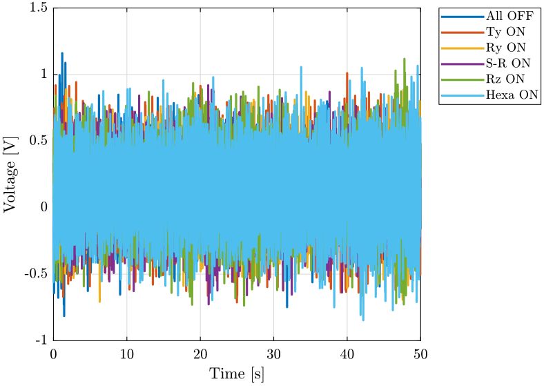
Figure 9: Comparison of the time domain data when turning off the control system of the stages - Geophone at the sample location

figure;
hold on;
plot(d_of(:, 3), d_of(:, 1), 'DisplayName', 'All OFF');
plot(d_ty(:, 3), d_ty(:, 1), 'DisplayName', 'Ty ON');
plot(d_ry(:, 3), d_ry(:, 1), 'DisplayName', 'Ry ON');
plot(d_sr(:, 3), d_sr(:, 1), 'DisplayName', 'S-R ON');
plot(d_rz(:, 3), d_rz(:, 1), 'DisplayName', 'Rz ON');
plot(d_he(:, 3), d_he(:, 1), 'DisplayName', 'Hexa ON');
hold off;
xlabel('Time [s]'); ylabel('Voltage [V]');
xlim([0, 50]);
legend('Location', 'bestoutside');

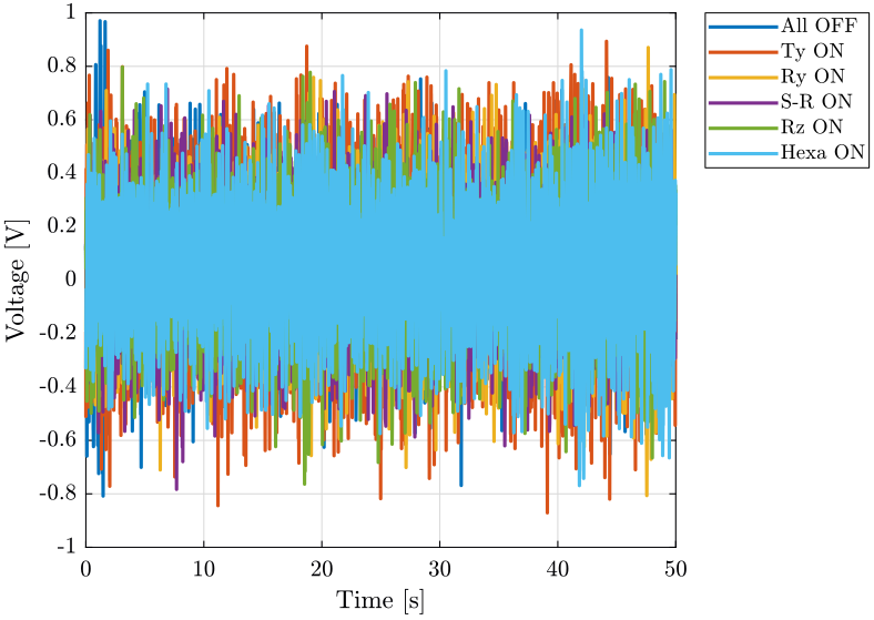
Figure 10: Comparison of the time domain data when turning off the control system of the stages - Geophone on the marble

2.4 Analysis - Frequency Domain

dt = d_of(2, 3) - d_of(1, 3);

Fs = 1/dt;
win = hanning(ceil(10*Fs));

2.4.1 Vibrations at the sample location

First, we compute the Power Spectral Density of the signals coming from the Geophone located at the sample location.

[px_of, f] = pwelch(d_of(:, 2), win, [], [], Fs);
[px_ty, ~] = pwelch(d_ty(:, 2), win, [], [], Fs);
[px_ry, ~] = pwelch(d_ry(:, 2), win, [], [], Fs);
[px_sr, ~] = pwelch(d_sr(:, 2), win, [], [], Fs);
[px_rz, ~] = pwelch(d_rz(:, 2), win, [], [], Fs);
[px_he, ~] = pwelch(d_he(:, 2), win, [], [], Fs);

And we compare all the signals (figures 11 and 12).

figure;
hold on;
plot(f, sqrt(px_of), 'DisplayName', 'All OFF');
plot(f, sqrt(px_ty), 'DisplayName', 'Ty ON');
plot(f, sqrt(px_ry), 'DisplayName', 'Ry ON');
plot(f, sqrt(px_sr), 'DisplayName', 'S-R ON');
plot(f, sqrt(px_rz), 'DisplayName', 'Rz ON');
plot(f, sqrt(px_he), 'DisplayName', 'Hexa ON');
hold off;
set(gca, 'xscale', 'log');
set(gca, 'yscale', 'log');
xlabel('Frequency [Hz]'); ylabel('Amplitude Spectral Density $\left[\frac{V}{\sqrt{Hz}}\right]$')
xlim([0.1, 500]);
legend('Location', 'southwest');

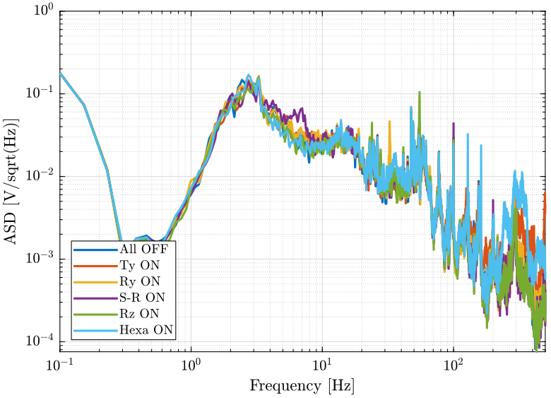
Figure 11: Amplitude Spectral Density of the signal coming from the top geophone

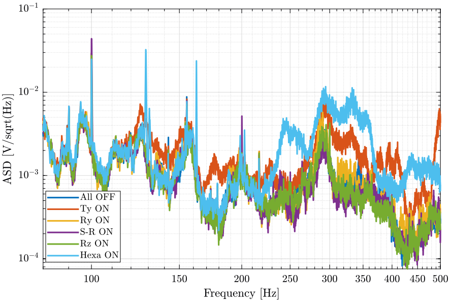
Figure 12: Amplitude Spectral Density of the signal coming from the top geophone (zoom at high frequencies)

2.4.2 Vibrations on the marble

Now we plot the same curves for the geophone located on the marble.

[px_of, f] = pwelch(d_of(:, 1), win, [], [], Fs);
[px_ty, ~] = pwelch(d_ty(:, 1), win, [], [], Fs);
[px_ry, ~] = pwelch(d_ry(:, 1), win, [], [], Fs);
[px_sr, ~] = pwelch(d_sr(:, 1), win, [], [], Fs);
[px_rz, ~] = pwelch(d_rz(:, 1), win, [], [], Fs);
[px_he, ~] = pwelch(d_he(:, 1), win, [], [], Fs);

And we compare the Amplitude Spectral Densities (figures 13 and 14)

figure;
hold on;
plot(f, sqrt(px_of), 'DisplayName', 'All OFF');
plot(f, sqrt(px_ty), 'DisplayName', 'Ty ON');
plot(f, sqrt(px_ry), 'DisplayName', 'Ry ON');
plot(f, sqrt(px_sr), 'DisplayName', 'S-R ON');
plot(f, sqrt(px_rz), 'DisplayName', 'Rz ON');
plot(f, sqrt(px_he), 'DisplayName', 'Hexa ON');
hold off;
set(gca, 'xscale', 'log');
set(gca, 'yscale', 'log');
xlabel('Frequency [Hz]'); ylabel('Amplitude Spectral Density $\left[\frac{V}{\sqrt{Hz}}\right]$')
xlim([0.1, 500]);
legend('Location', 'northeast');

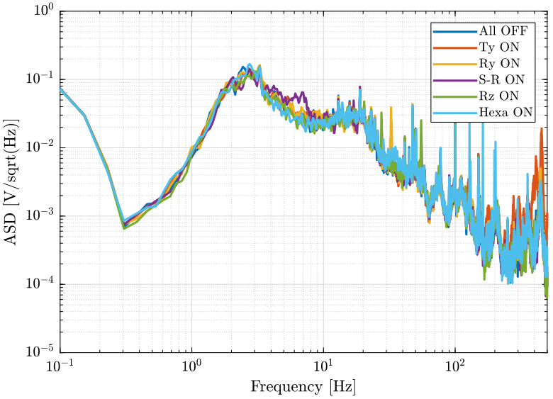
Figure 13: Amplitude Spectral Density of the signal coming from geophone located on the marble

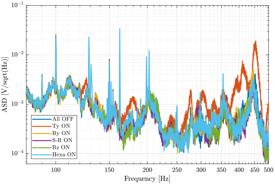
Figure 14: Amplitude Spectral Density of the signal coming from the geophone located on the marble (zoom at high frequencies)

2.5 Conclusion

The Ty stage induces vibrations of the marble and at the sample location above 100Hz
The hexapod stage induces vibrations at the sample position above 220Hz

3 Effect of the Symetrie Driver

All the files (data and Matlab scripts) are accessible here.

3.1 Experimental Setup

We here measure the signals of two geophones:

One is located on top of the Sample platform
One is located on the marble

The signal from the top geophone does go trought the slip-ring.

All the control systems are turned OFF except the Hexapod one.

Each measurement are done during 100s.

The settings of the voltage amplifier are:

DC
60dB
1kHz

A first order low pass filter with a cut-off frequency of 1kHz is added before the voltage amplifier.

The measurements are:

meas_018.mat: Hexapod's driver on the granite
meas_019.mat: Hexapod's driver on the ground

Each of the mat file contains one array data with 3 columns:

Column number	Description
1	Geophone - Marble
2	Geophone - Sample
3	Time

3.2 Load data

We load the data of the z axis of two geophones.

d_18 = load('mat/data_018.mat', 'data'); d_18 = d_18.data;
d_19 = load('mat/data_019.mat', 'data'); d_19 = d_19.data;

3.3 Analysis - Time Domain

figure;
hold on;
plot(d_19(:, 3), d_19(:, 1), 'DisplayName', 'Driver - Ground');
plot(d_18(:, 3), d_18(:, 1), 'DisplayName', 'Driver - Granite');
hold off;
xlabel('Time [s]'); ylabel('Voltage [V]');
xlim([0, 50]);
legend('Location', 'bestoutside');

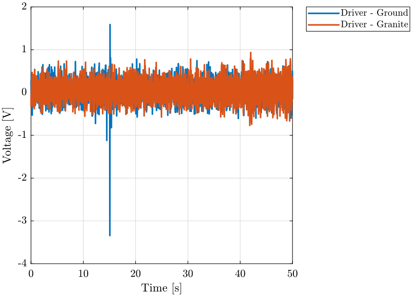
Figure 15: Comparison of the time domain data when turning off the control system of the stages - Geophone at the sample location

3.4 Analysis - Frequency Domain

dt = d_18(2, 3) - d_18(1, 3);

Fs = 1/dt;
win = hanning(ceil(10*Fs));

3.4.1 Vibrations at the sample location

First, we compute the Power Spectral Density of the signals coming from the Geophone located at the sample location.

[px_18, f] = pwelch(d_18(:, 1), win, [], [], Fs);
[px_19, ~] = pwelch(d_19(:, 1), win, [], [], Fs);

figure;
hold on;
plot(f, sqrt(px_19), 'DisplayName', 'Driver - Ground');
plot(f, sqrt(px_18), 'DisplayName', 'Driver - Granite');
hold off;
set(gca, 'xscale', 'log');
set(gca, 'yscale', 'log');
xlabel('Frequency [Hz]'); ylabel('Amplitude Spectral Density $\left[\frac{V}{\sqrt{Hz}}\right]$')
xlim([0.1, 500]);
legend('Location', 'southwest');

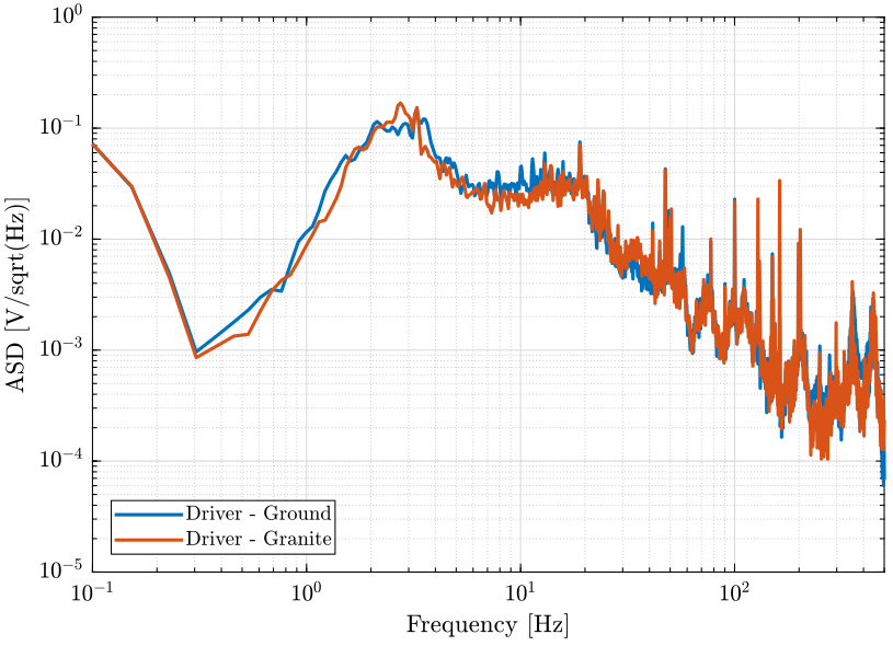
Figure 16: Amplitude Spectral Density of the signal coming from the top geophone

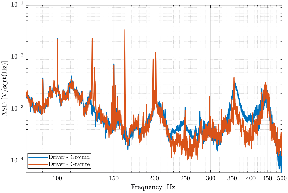
Figure 17: Amplitude Spectral Density of the signal coming from the top geophone (zoom at high frequencies)

3.5 Conclusion

Even tough the Hexapod's driver vibrates quite a lot, it does not generate significant vibrations of the granite when either placed on the granite or on the ground.

4 Transfer function from one stage to the other

All the files (data and Matlab scripts) are accessible here.

4.1 Experimental Setup

For all the measurements in this section:

all the control stages are OFF.
the measurements are on the \(z\) direction

4.1.1 From Marble to Ty - `mat/meas_010.mat`

One geophone is on the marble, one is on the Ty stage (see figures 18, 19 and 20).

The data array contains the following columns:

Column	Description
1	Ground
2	Ty
3	Time

Figure 18: Setup with one geophone on the marble and one on top of the translation stage

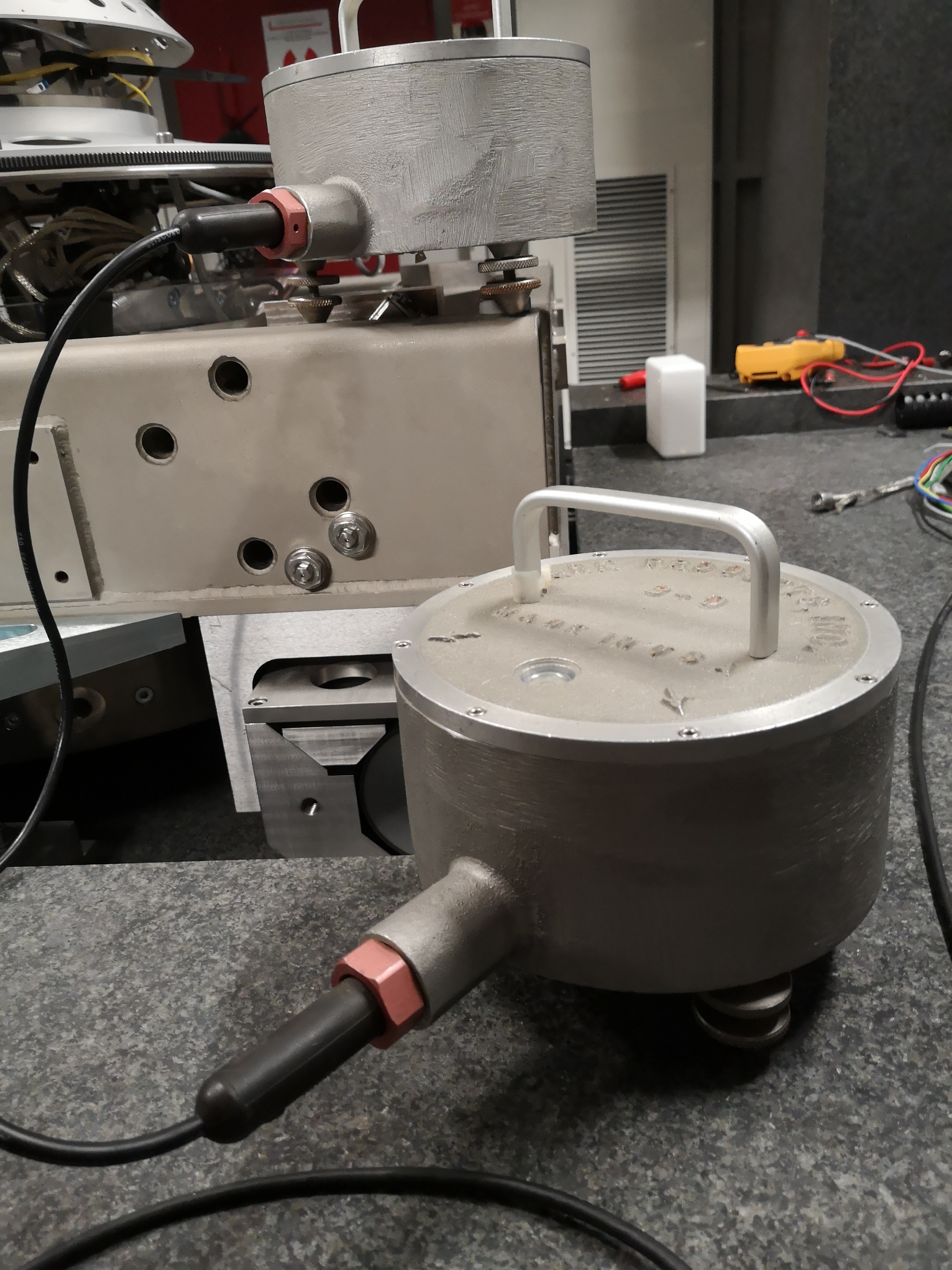
Figure 19: Setup with one geophone on the marble and one on top of the translation stage - Close up view

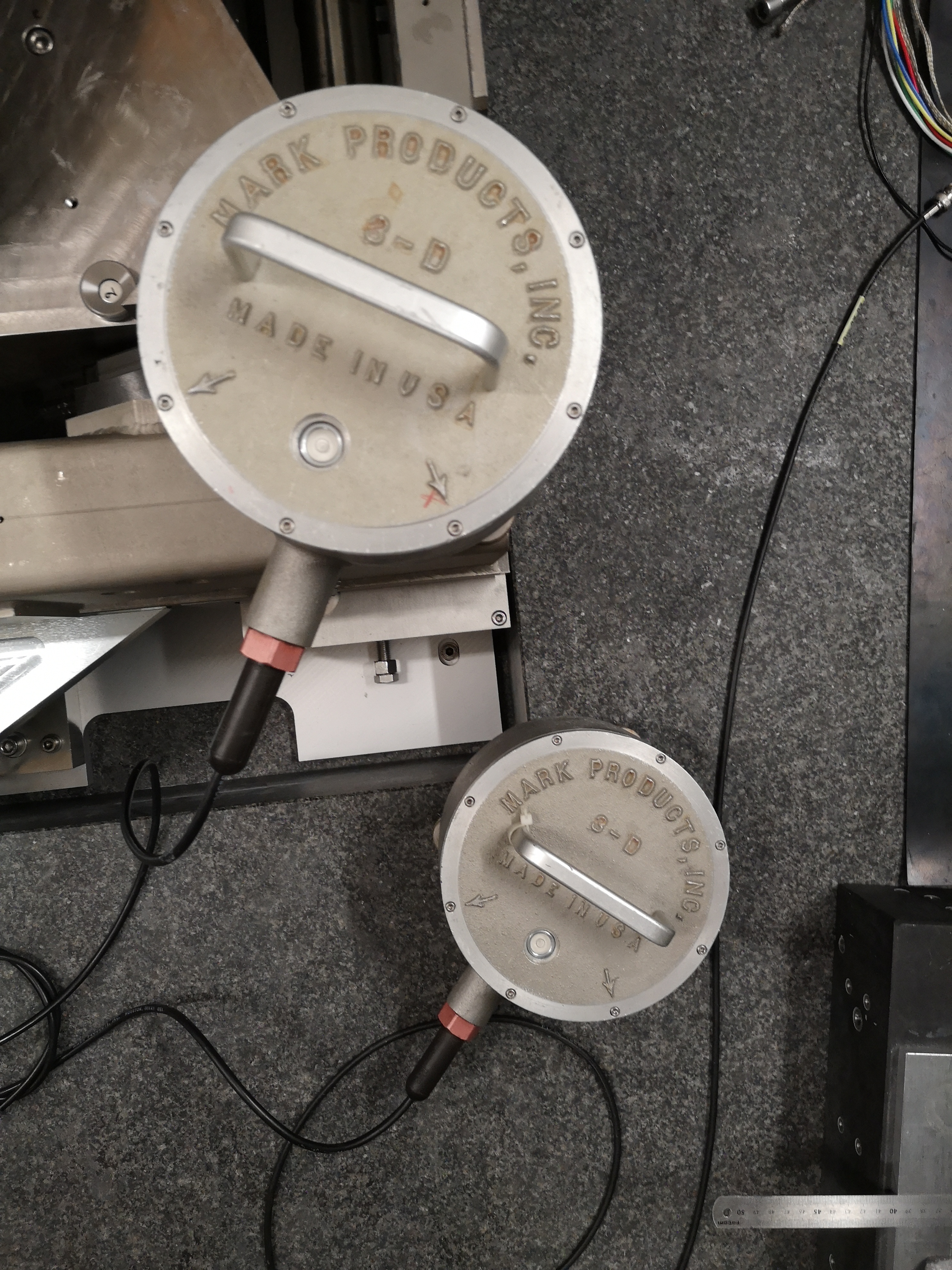
Figure 20: Setup with one geophone on the marble and one on top of the translation stage - Top view

4.1.2 From Marble to Ry - `mat/meas_011.mat`

One geophone is on the marble, one is on the Ry stage (see figure 21)

The data array contains the following columns:

Column	Description
1	Ground
2	Ry
3	Time

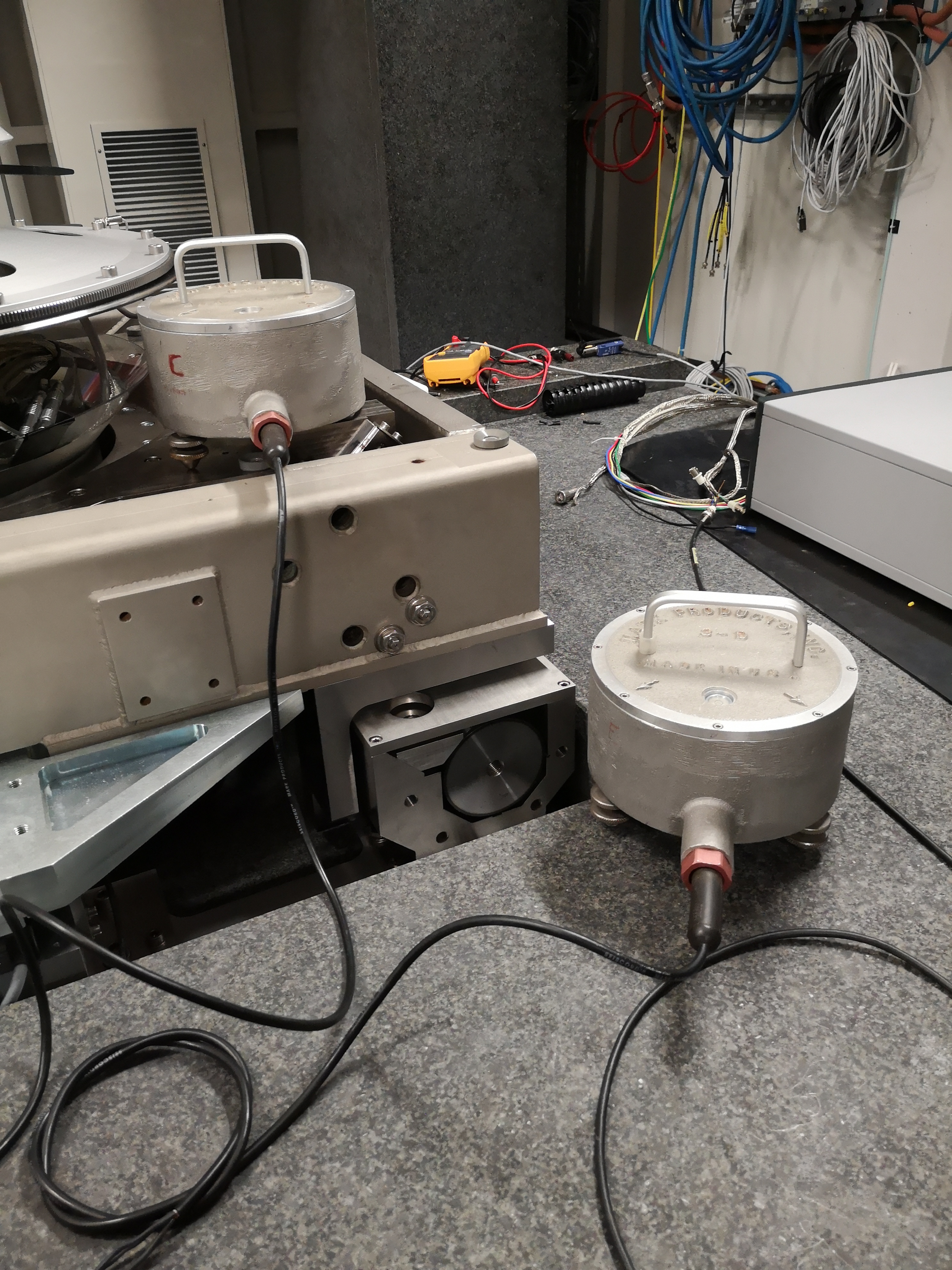
Figure 21: Setup with one geophone on the marble and one on top of the Tilt Stage

4.1.3 From Ty to Ry - `mat/meas_012.mat`

One geophone is on the Ty stage, one is on the Ry stage (see figures 22, 23 and 24) One geophone on the Ty stage, one geophone on the Ry stage.

The data array contains the following columns:

Column	Description
1	Ty
2	Ry
3	Time

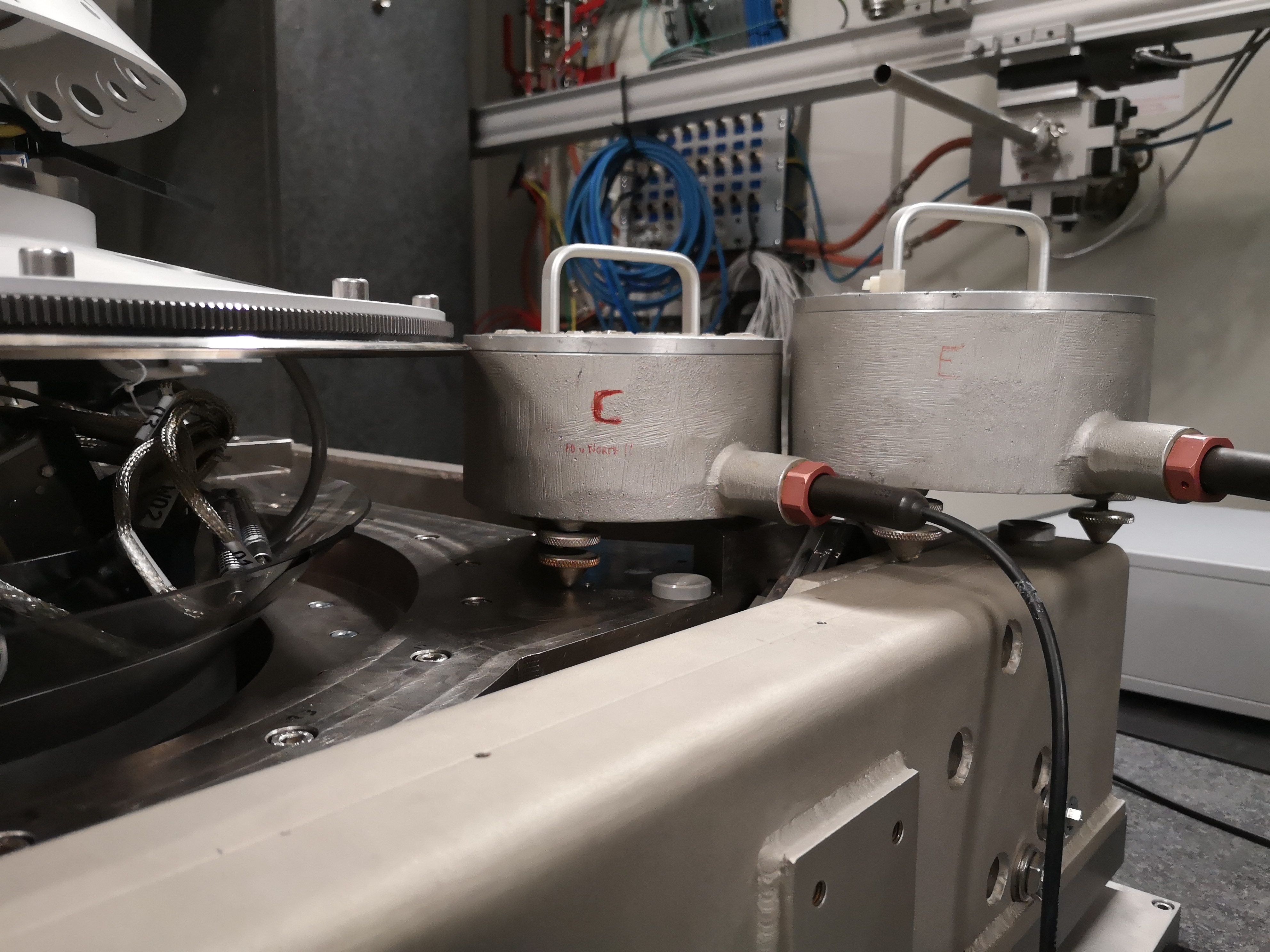
Figure 22: Setup with one geophone on the translation stage and one on top of the Tilt Stage

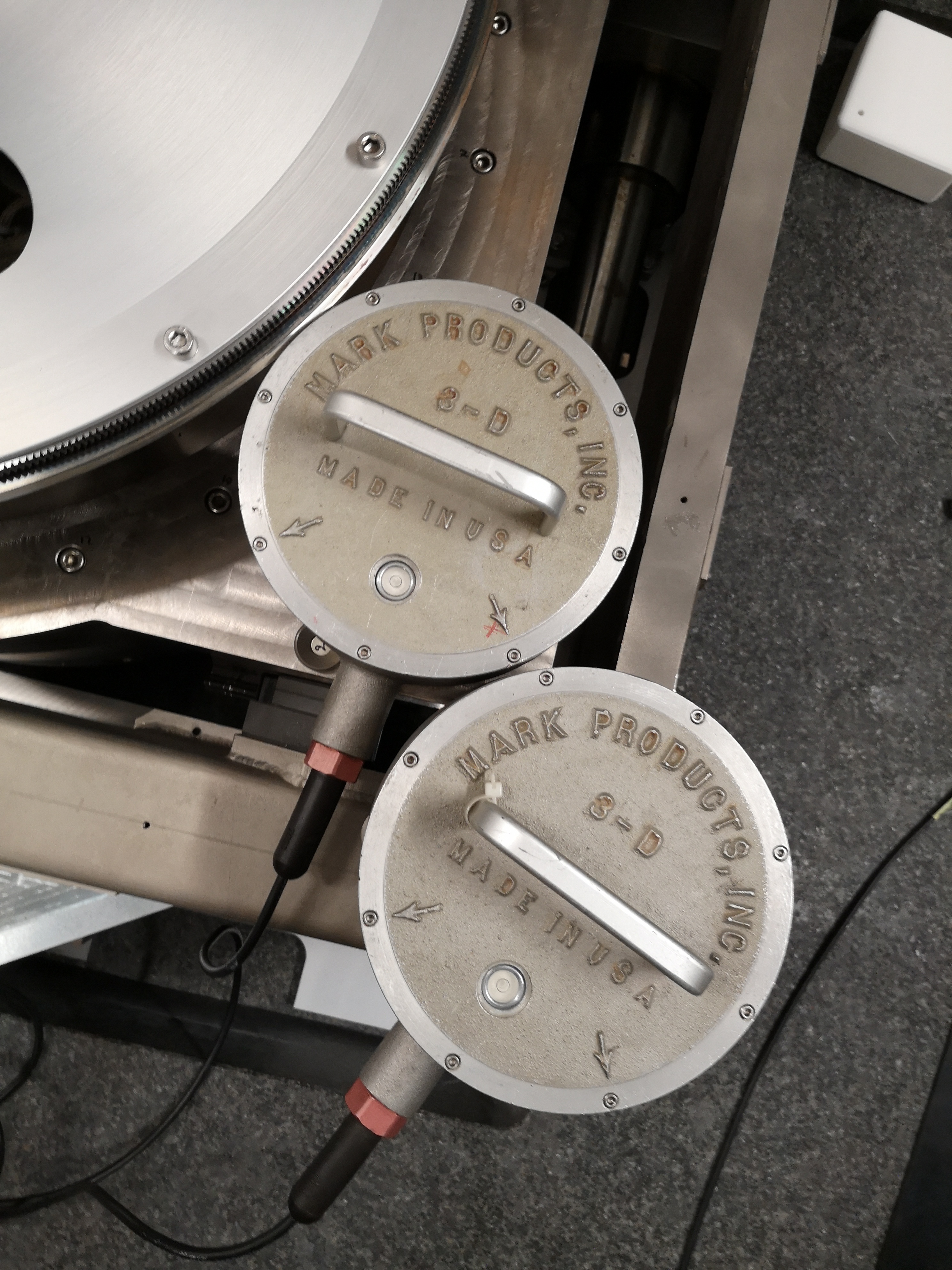
Figure 23: Setup with one geophone on the translation stage and one on top of the Tilt Stage - Top view

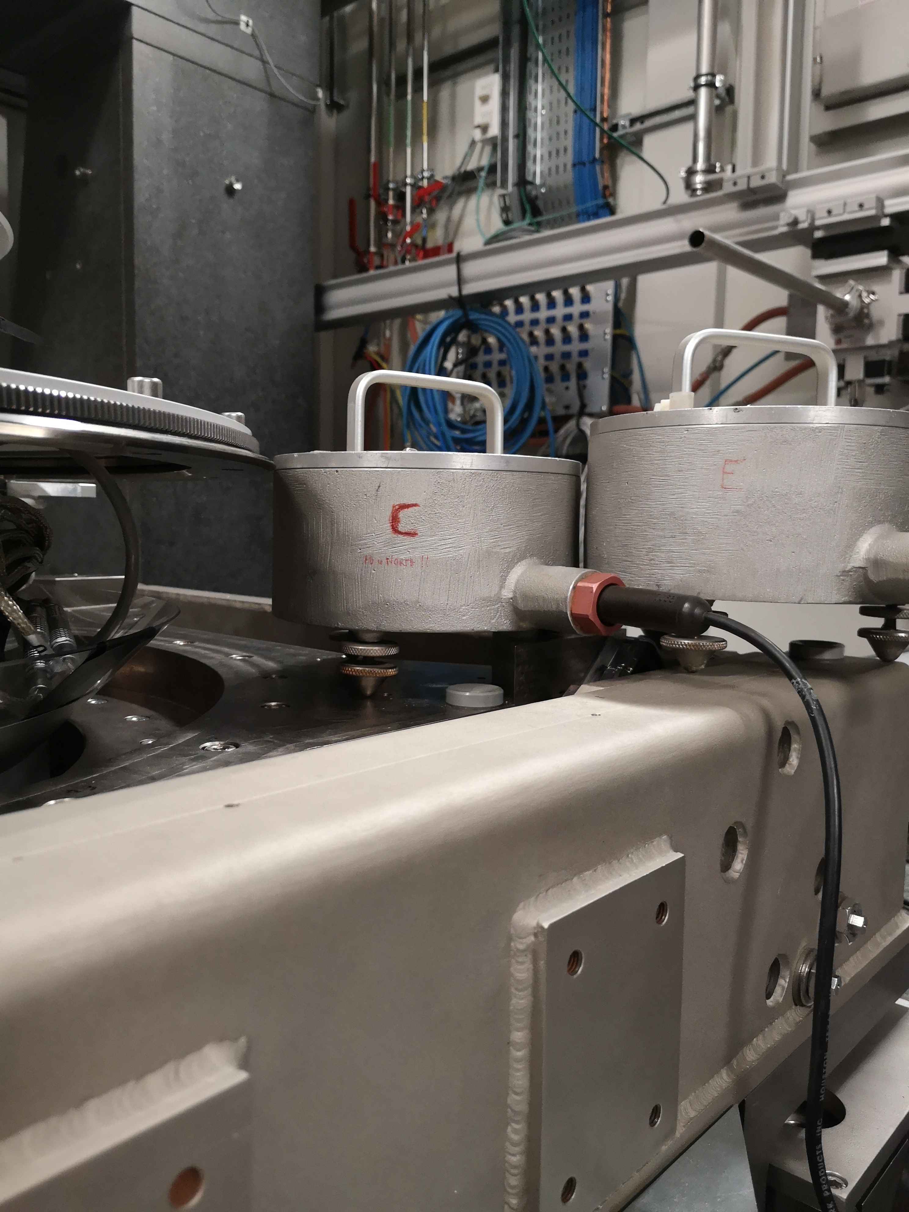
Figure 24: Setup with one geophone on the translation stage and one on top of the Tilt Stage - Close up view

4.2 Load data

We load the data of the z axis of two geophones.

m_ty  = load('mat/data_010.mat', 'data'); m_ty  = m_ty.data;
m_ry  = load('mat/data_011.mat', 'data'); m_ry  = m_ry.data;
ty_ry = load('mat/data_012.mat', 'data'); ty_ry = ty_ry.data;

4.3 Analysis - Time Domain

First, we can look at the time domain data.

figure;
hold on;
plot(m_ty(:, 3), m_ty(:, 1), 'DisplayName', 'Marble');
plot(m_ty(:, 3), m_ty(:, 2), 'DisplayName', 'Ty');
hold off;
xlabel('Time [s]'); ylabel('Voltage [V]');
legend('Location', 'northeast');
xlim([0, 500]);

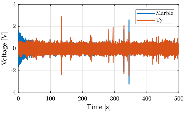
Figure 25: Time domain - Marble and translation stage

figure;
hold on;
plot(m_ry(:, 3), m_ry(:, 1), 'DisplayName', 'Marble');
plot(m_ry(:, 3), m_ry(:, 2), 'DisplayName', 'Ty');
hold off;
xlabel('Time [s]'); ylabel('Voltage [V]');
legend('Location', 'northeast');
xlim([0, 500]);

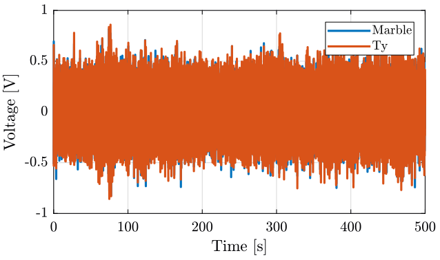
Figure 26: Time domain - Marble and tilt stage

figure;
hold on;
plot(ty_ry(:, 3), ty_ry(:, 1), 'DisplayName', 'Ty');
plot(ty_ry(:, 3), ty_ry(:, 2), 'DisplayName', 'Ry');
hold off;
xlabel('Time [s]'); ylabel('Voltage [V]');
legend('Location', 'northeast');
xlim([0, 500]);

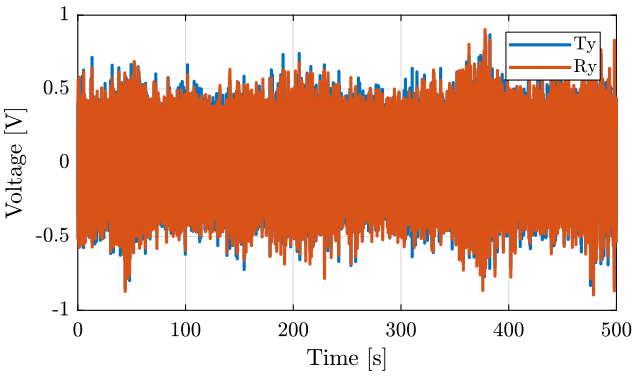
Figure 27: Time domain - Translation stage and tilt stage

4.4 Analysis - Frequency Domain

dt = m_ty(2, 3) - m_ty(1, 3);

Fs = 1/dt;
win = hanning(ceil(1*Fs));

First, we compute the transfer function estimate between the two geophones for the 3 experiments (figure 28). We also plot their coherence (figure 29).

[T_m_ty,  f] = tfestimate(m_ty(:, 1),  m_ty(:, 2),  win, [], [], Fs);
[T_m_ry,  ~] = tfestimate(m_ry(:, 1),  m_ry(:, 2),  win, [], [], Fs);
[T_ty_ry, ~] = tfestimate(ty_ry(:, 1), ty_ry(:, 2), win, [], [], Fs);

figure;
ax1 = subplot(2, 1, 1);
hold on;
plot(f, abs(T_m_ty),  'DisplayName', 'Marble - Ty');
plot(f, abs(T_m_ry),  'DisplayName', 'Marble - Ry');
plot(f, abs(T_ty_ry), 'DisplayName', 'Ty - Ry');
hold off;
set(gca, 'xscale', 'log'); set(gca, 'yscale', 'log');
set(gca, 'XTickLabel',[]);
ylabel('Magnitude');
legend('Location', 'northwest');

ax2 = subplot(2, 1, 2);
hold on;
plot(f, mod(180+180/pi*phase(T_m_ty),  360)-180);
plot(f, mod(180+180/pi*phase(T_m_ry),  360)-180);
plot(f, mod(180+180/pi*phase(T_ty_ry), 360)-180);
hold off;
set(gca, 'xscale', 'log');
ylim([-180, 180]);
yticks([-180, -90, 0, 90, 180]);
xlabel('Frequency [Hz]'); ylabel('Phase');

linkaxes([ax1,ax2],'x');
xlim([10, 500]);

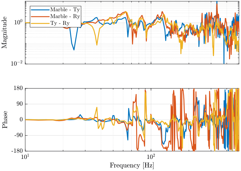
Figure 28: Transfer function from the first geophone to the second geophone for the three experiments

[coh_m_ty,  f] = mscohere(m_ty(:, 1),  m_ty(:, 2),  win, [], [], Fs);
[coh_m_ry,  ~] = mscohere(m_ry(:, 1),  m_ry(:, 2),  win, [], [], Fs);
[coh_ty_ry, ~] = mscohere(ty_ry(:, 1), ty_ry(:, 2), win, [], [], Fs);

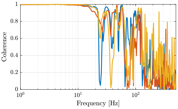
Figure 29: Coherence between the two geophones for the three experiments

4.5 Conclusion

These measurements are not relevant.

Measurements

Table of Contents

1 Effect of all the control systems on the Sample vibrations

1.1 Experimental Setup

1.2 Load data

1.3 Analysis - Time Domain

1.4 Analysis - Frequency Domain

1.4.1 Vibrations at the sample location

1.4.2 Vibrations on the marble

1.5 Effect of the control system on the transmissibility from ground to sample

1.6 Conclusion

2 Effect of all the control systems on the Sample vibrations - One stage at a time

2.1 Experimental Setup

2.2 Load data

2.3 Analysis - Time Domain

2.4 Analysis - Frequency Domain

2.4.1 Vibrations at the sample location

2.4.2 Vibrations on the marble

2.5 Conclusion

3 Effect of the Symetrie Driver

3.1 Experimental Setup

3.2 Load data

3.3 Analysis - Time Domain

3.4 Analysis - Frequency Domain

3.4.1 Vibrations at the sample location

3.5 Conclusion

4 Transfer function from one stage to the other

4.1 Experimental Setup

4.1.1 From Marble to Ty - mat/meas_010.mat

4.1.2 From Marble to Ry - mat/meas_011.mat

4.1.3 From Ty to Ry - mat/meas_012.mat

4.2 Load data

4.3 Analysis - Time Domain

4.4 Analysis - Frequency Domain

4.5 Conclusion

4.1.1 From Marble to Ty - `mat/meas_010.mat`

4.1.2 From Marble to Ry - `mat/meas_011.mat`

4.1.3 From Ty to Ry - `mat/meas_012.mat`