Measurements On the Slip-Ring
Table of Contents
We determine if the slip-ring add some noise to the signal when it is turning:
- Section 1:
- Noise is generated by the Speedgoat DAC and goes trough the slip-ring two times
- We measure the signal when it is OFF, ON but not turning and ON and turning
- However, the measurement is limited by the ADC noise
- Section 2:
- Voltage amplifiers are added, and the same measurements are done
- However, the voltage amplifiers are saturating because of high frequency noise
- Section 3:
- Low pass filter are added at the input of the voltage amplifier and the same measurement is done
1 Effect of the rotation of the Slip-Ring - Noise
All the files (data and Matlab scripts) are accessible here.
1.1 Measurement Description
Setup: Random Signal is generated by one SpeedGoat DAC.
The signal going out of the DAC is split into two:
- one BNC cable is directly connected to one ADC of the SpeedGoat
- one BNC cable goes two times in the Slip-Ring (from bottom to top and then from top to bottom) and then is connected to one ADC of the SpeedGoat
All the stages are turned OFF except the Slip-Ring.
Goal: The goal is to determine if the signal is altered when the spindle is rotating.
Measurements:
| Data File | Description |
|---|---|
mat/data_001.mat |
Slip-ring not turning but ON |
mat/data_002.mat |
Slip-ring turning at 1rpm |
For each measurement, the measured signals are:
| Variable | Description |
|---|---|
t |
Time vector |
x1 |
Direct signal |
x2 |
Signal going through the Slip-Ring |
1.2 Load data
We load the data of the z axis of two geophones.
sr_off = load('mat/data_001.mat', 't', 'x1', 'x2');
sr_on  = load('mat/data_002.mat', 't', 'x1', 'x2');
1.3 Analysis
Let’s first look at the signal produced by the DAC (figure 1).
figure;
hold on;
plot(sr_on.t,  sr_on.x1);
hold off;
xlabel('Time [s]'); ylabel('Voltage [V]');
xlim([0 10]);
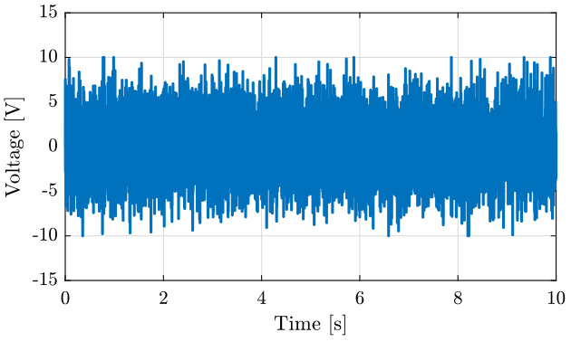
Figure 1: Random signal produced by the DAC
We now look at the difference between the signal directly measured by the ADC and the signal that goes through the slip-ring (figure 2).
figure;
hold on;
plot(sr_on.t,  sr_on.x1  -  sr_on.x2,  'DisplayName', 'Slip-Ring - $\omega = 1rpm$');
plot(sr_off.t, sr_off.x1 - sr_off.x2,'DisplayName', 'Slip-Ring off');
hold off;
xlabel('Time [s]'); ylabel('Voltage [V]');
xlim([0 10]);
legend('Location', 'northeast');
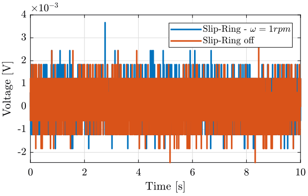
Figure 2: Alteration of the signal when the slip-ring is turning
dt = sr_on.t(2) - sr_on.t(1);
Fs = 1/dt; % [Hz]

win = hanning(ceil(1*Fs));
[pxx_on,  f] = pwelch(sr_on.x1  - sr_on.x2,  win, [], [], Fs);
[pxx_off, ~] = pwelch(sr_off.x1 - sr_off.x2, win, [], [], Fs);
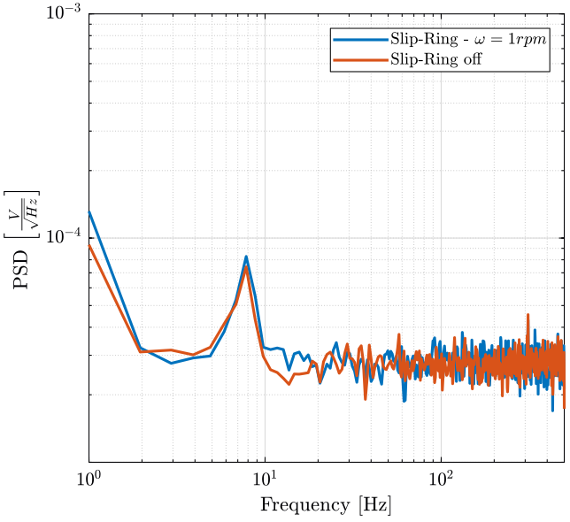
Figure 3: ASD of the measured noise
1.4 Conclusion
- The measurement is mostly limited by the resolution of the Speedgoat DAC (16bits over \(\pm 10 V\))
- In section 2, the same measurement is done but voltage amplifiers are added to amplify the noise
2 Measure of the noise induced by the Slip-Ring using voltage amplifiers - Noise
All the files (data and Matlab scripts) are accessible here.
2.1 Measurement Description
Goal:
- Determine the noise induced by the slip-ring when turned ON and when rotating
Setup:
- 0V is generated by one Speedgoat DAC
- Using a T, one part goes directly to one Speedgoat ADC
- The other part goes to the slip-ring 2 times and then to one voltage amplifier before going to the ADC
- The parameters of the Voltage Amplifier are:
- gain of 80dB
- AC/DC option to AC (it adds an high pass filter at 1.5Hz at the input of the voltage amplifier)
- Output Low pass filter set at 1kHz
- Every stage of the station is OFF
First column: Direct measure Second column: Slip-ring measure
Measurements:
| Data File | Description |
|---|---|
mat/data_008.mat |
Slip-Ring OFF |
mat/data_009.mat |
Slip-Ring ON |
mat/data_010.mat |
Slip-Ring ON and omega=6rpm |
mat/data_011.mat |
Slip-Ring ON and omega=60rpm |
Each of the measurement mat file contains one data array with 3 columns:
| Column number | Description |
|---|---|
| 1 | Signal going directly to the ADC |
| 2 | Signal going through the Slip-Ring |
| 3 | Time |
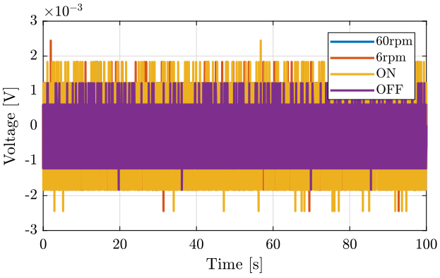
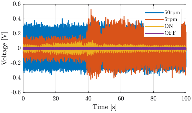
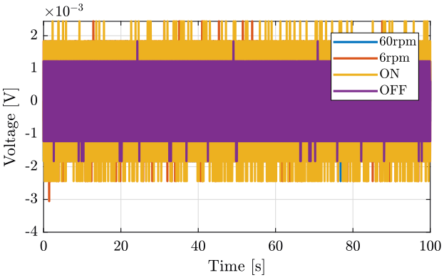
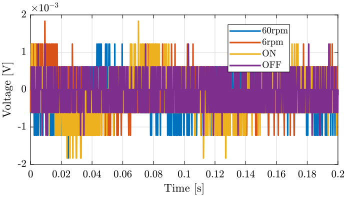
Figure 4: Slip-Ring rotating at 6rpm
Figure 5: Slip-Ring rotating at 60rpm
2.2 Load data
We load the data of the z axis of two geophones.
sr_off = load('mat/data_008.mat', 'data'); sr_off = sr_off.data;
sr_on  = load('mat/data_009.mat', 'data'); sr_on  = sr_on.data;
sr_6r  = load('mat/data_010.mat', 'data'); sr_6r  = sr_6r.data;
sr_60r = load('mat/data_011.mat', 'data'); sr_60r = sr_60r.data;
2.3 Time Domain
2.4 Frequency Domain
We first compute some parameters that will be used for the PSD computation.
dt = sr_off(2, 3)-sr_off(1, 3);

Fs = 1/dt; % [Hz]

win = hanning(ceil(10*Fs));
Then we compute the Power Spectral Density using pwelch function.
[pxdir, f] = pwelch(sr_off(:, 1), win, [], [], Fs);
[pxoff, ~] = pwelch(sr_off(:, 2), win, [], [], Fs);
[pxon,  ~] = pwelch(sr_on(:, 2),  win, [], [], Fs);
[px6r,  ~] = pwelch(sr_6r(:, 2),  win, [], [], Fs);
[px60r, ~] = pwelch(sr_60r(:, 2), win, [], [], Fs);
And we plot the ASD of the measured signals (figure 8);
figure;
hold on;
plot(f, sqrt(pxoff), 'DisplayName', 'OFF');
plot(f, sqrt(pxon),  'DisplayName', 'ON');
plot(f, sqrt(px6r),  'DisplayName', '6rpm');
plot(f, sqrt(px60r), 'DisplayName', '60rpm');
plot(f, sqrt(pxdir), 'k-', 'DisplayName', 'Direct');
hold off;
set(gca, 'xscale', 'log');
set(gca, 'yscale', 'log');
xlabel('Frequency [Hz]'); ylabel('ASD of the measured Voltage $\left[\frac{V}{\sqrt{Hz}}\right]$')
legend('Location', 'northeast');
xlim([0.1, 500]);
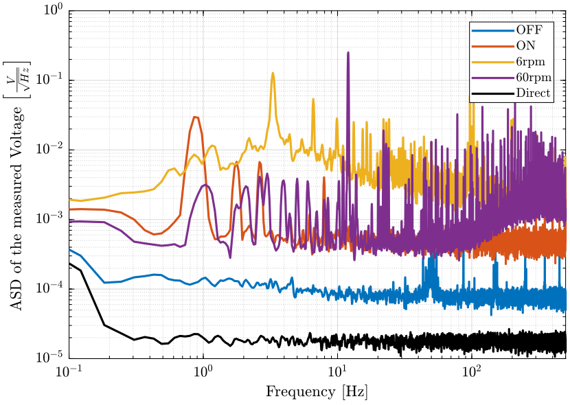
Figure 8: Comparison of the ASD of the measured signals when the slip-ring is ON, OFF and turning
Questions:
- Why is there some sharp peaks? Can this be due to aliasing?
- It is possible that the amplifiers were saturating during the measurements. This saturation could be due to high frequency noise.
2.5 Conclusion
- The measurements are re-done using an additional low pass filter at the input of the voltage amplifier
3 Measure of the noise induced by the Slip-Ring rotation - LPF added
All the files (data and Matlab scripts) are accessible here.
3.1 Measurement description
Setup: Voltage amplifier:
- 60db
- AC
- 1kHz
Additionnal LPF at 1kHz
Goal:
Measurements:
Three measurements are done:
| Measurement File | Description |
|---|---|
mat/data_030.mat |
All off |
mat/data_031.mat |
Slip-Ring on |
mat/data_032.mat |
Slip-Ring 6rpm |
mat/data_033.mat |
Slip-Ring 60rpm |
Each of the measurement mat file contains one data array with 3 columns:
| Column number | Description |
|---|---|
| 1 | Direct Measure |
| 2 | Slip-Ring |
| 3 | Time |
3.2 Load data
We load the data of the z axis of two geophones.
sr_of = load('mat/data_030.mat', 'data'); sr_of = sr_of.data;
sr_on = load('mat/data_031.mat', 'data'); sr_on = sr_on.data;
sr_6r = load('mat/data_032.mat', 'data'); sr_6r = sr_6r.data;
sr_60 = load('mat/data_033.mat', 'data'); sr_60 = sr_60.data;
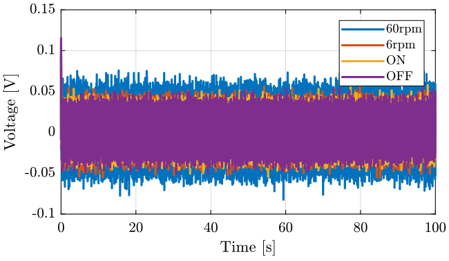
3.3 Time Domain
3.4 Frequency Domain - Direct Signal
We first compute some parameters that will be used for the PSD computation.
dt = sr_of(2, 3)-sr_of(1, 3);

Fs = 1/dt; % [Hz]

win = hanning(ceil(10*Fs));
Then we compute the Power Spectral Density using pwelch function.
[px_d_of, f] = pwelch(sr_of(:, 1), win, [], [], Fs);
[px_d_on, ~] = pwelch(sr_on(:, 1), win, [], [], Fs);
[px_d_6r, ~] = pwelch(sr_6r(:, 1), win, [], [], Fs);
[px_d_60, ~] = pwelch(sr_60(:, 1), win, [], [], Fs);
figure;
hold on;
plot(f, sqrt(px_d_of), 'DisplayName', 'OFF');
plot(f, sqrt(px_d_on), 'DisplayName', 'ON');
plot(f, sqrt(px_d_6r), 'DisplayName', '6rpm');
plot(f, sqrt(px_d_60), 'DisplayName', '60rpm');
hold off;
set(gca, 'xscale', 'log');
set(gca, 'yscale', 'log');
xlabel('Frequency [Hz]'); ylabel('ASD of the measured Voltage $\left[\frac{V}{\sqrt{Hz}}\right]$')
legend('Location', 'northeast');
xlim([0.1, 5000]);
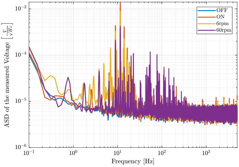
Figure 12: Amplitude Spectral Density of the signal going directly to the ADC
3.5 Frequency Domain - Slip-Ring Signal
[px_sr_of, f] = pwelch(sr_of(:, 2), win, [], [], Fs);
[px_sr_on, ~] = pwelch(sr_on(:, 2), win, [], [], Fs);
[px_sr_6r, ~] = pwelch(sr_6r(:, 2), win, [], [], Fs);
[px_sr_60, ~] = pwelch(sr_60(:, 2), win, [], [], Fs);
figure;
hold on;
plot(f, sqrt(px_sr_of), 'DisplayName', 'OFF');
plot(f, sqrt(px_sr_on), 'DisplayName', 'ON');
plot(f, sqrt(px_sr_6r), 'DisplayName', '6rpm');
plot(f, sqrt(px_sr_60), 'DisplayName', '60rpm');
plot(f, sqrt(px_d_of), '-k', 'DisplayName', 'Direct');
hold off;
set(gca, 'xscale', 'log');
set(gca, 'yscale', 'log');
xlabel('Frequency [Hz]'); ylabel('ASD of the measured Voltage $\left[\frac{V}{\sqrt{Hz}}\right]$')
legend('Location', 'northeast');
xlim([0.1, 5000]);
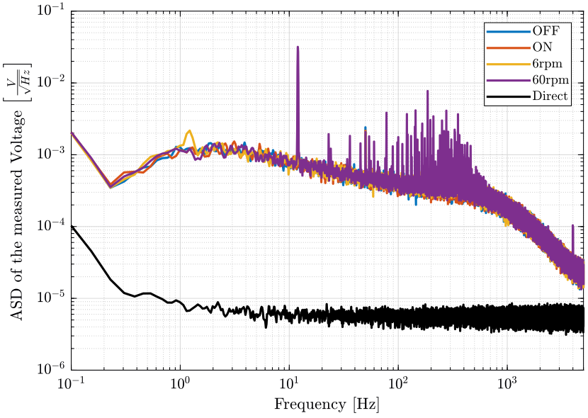
Figure 13: Amplitude Spectral Density of the signal going through the slip-ring
3.6 Conclusion
- We observe peaks at 12Hz and its harmonics for the signal going through the slip-ring when it is turning at 60rpm.
- Apart from that, the noise of the signal is the same when the slip-ring is off/on and turning
- The noise of the signal going through the slip-ring is much higher that the direct signal from the DAC to the ADC
- A peak is obverse at 11.5Hz on the direct signal as soon as the slip-ring is turned ON. Can this be due to high frequency noise and Aliasing? As there is no LPF to filter the noise on the direct signal, this effect could be more visible on the direct signal.