Vibrations induced by the Slip-Ring and the Spindle
Table of Contents
1 Experimental Setup
Setup: All the stages are OFF.
Two geophone are use:
- One on the marble (corresponding to the first column in the data)
- One at the sample location (corresponding to the second column in the data)
Two voltage amplifiers are used, their setup is:
- gain of 60dB
- AC/DC switch on AC
- Low pass filter at 1kHz
A first order low pass filter is also added at the input of the voltage amplifiers.
Goal:
- Identify the vibrations induced by the rotation of the Slip-Ring and Spindle
Measurements: Three measurements are done:
| Measurement File | Description |
|---|---|
mat/data_024.mat |
All the stages are OFF |
mat/data_025.mat |
The slip-ring is ON and rotates at 6rpm. The spindle is OFF |
mat/data_026.mat |
The slip-ring and spindle are both ON. They are both turning at 6rpm |
Each of the measurement mat file contains one data array with 3 columns:
| Column number | Description |
|---|---|
| 1 | Geophone - Marble |
| 2 | Geophone - Sample |
| 3 | Time |
A movie showing the experiment is shown on figure 1.
Figure 1: Movie of the experiment, rotation speed is 6rpm
2 Data Analysis
All the files (data and Matlab scripts) are accessible here.
2.1 Load data
of = load('mat/data_024.mat', 'data'); of = of.data; % OFF
sr = load('mat/data_025.mat', 'data'); sr = sr.data; % Slip Ring
sp = load('mat/data_026.mat', 'data'); sp = sp.data; % Spindle
There is a sign error for the Geophone located on top of the Hexapod. The problem probably comes from the wiring in the Slip-Ring.
of(:, 2) = -of(:, 2);
sr(:, 2) = -sr(:, 2);
sp(:, 2) = -sp(:, 2);
2.2 Voltage to Velocity
We convert the measured voltage to velocity using the function voltageToVelocityL22 (accessible here).
gain = 60; % [dB]

of(:, 1) = voltageToVelocityL22(of(:, 1), of(:, 3), gain);
sr(:, 1) = voltageToVelocityL22(sr(:, 1), sr(:, 3), gain);
sp(:, 1) = voltageToVelocityL22(sp(:, 1), sp(:, 3), gain);

of(:, 2) = voltageToVelocityL22(of(:, 2), of(:, 3), gain);
sr(:, 2) = voltageToVelocityL22(sr(:, 2), sr(:, 3), gain);
sp(:, 2) = voltageToVelocityL22(sp(:, 2), sp(:, 3), gain);
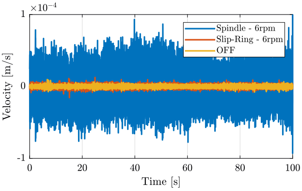
2.3 Time domain plots
figure;
hold on;
plot(sp(:, 3), sp(:, 1), 'DisplayName', 'Spindle - 6rpm');
plot(sr(:, 3), sr(:, 1), 'DisplayName', 'Slip-Ring - 6rpm');
plot(of(:, 3), of(:, 1), 'DisplayName', 'OFF');
hold off;
xlabel('Time [s]'); ylabel('Velocity [m/s]');
xlim([0, 100]);
legend('Location', 'northeast');
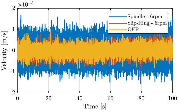
Figure 2: Velocity as measured by the geophone located on the marble - Time domain
figure;
hold on;
plot(sp(:, 3), sp(:, 2), 'DisplayName', 'Spindle and Slip-Ring');
plot(sr(:, 3), sr(:, 2), 'DisplayName', 'Only Slip-Ring');
plot(of(:, 3), of(:, 2), 'DisplayName', 'OFF');
hold off;
xlabel('Time [s]'); ylabel('Velocity [m/s]');
xlim([0, 100]);
legend('Location', 'northeast');
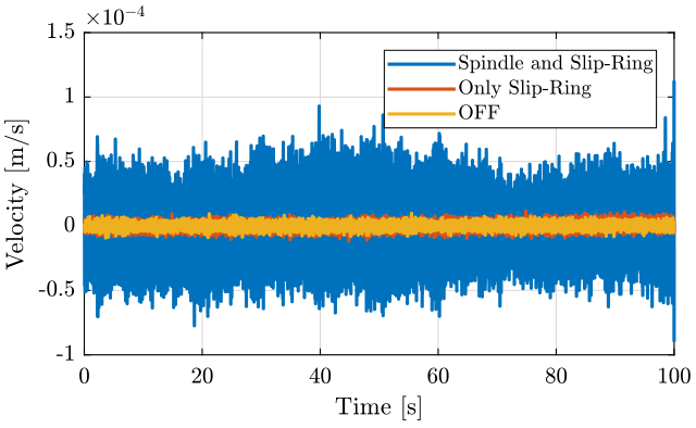
Figure 3: Velocity as measured by the geophone at the sample location - Time domain
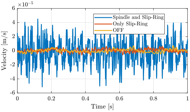
Figure 4: Velocity as measured by the geophone at the sample location - Time domain
2.4 Frequency Domain
We first compute some parameters that will be used for the PSD computation.
dt = of(2, 3)-of(1, 3); % [s]

Fs = 1/dt; % [Hz]

win = hanning(ceil(10*Fs)); % Window used
Then we compute the Power Spectral Density using pwelch function.
First for the geophone located on the marble
[pxof_m, f] = pwelch(of(:, 1), win, [], [], Fs);
[pxsr_m, ~] = pwelch(sr(:, 1), win, [], [], Fs);
[pxsp_m, ~] = pwelch(sp(:, 1), win, [], [], Fs);
And for the geophone located at the sample position.
[pxof_s, ~] = pwelch(of(:, 2), win, [], [], Fs);
[pxsr_s, ~] = pwelch(sr(:, 2), win, [], [], Fs);
[pxsp_s, ~] = pwelch(sp(:, 2), win, [], [], Fs);
And we plot the ASD of the measured velocities:
figure;
hold on;
plot(f, sqrt(pxsp_m), 'DisplayName', 'Spindle - 6rpm');
plot(f, sqrt(pxsr_m), 'DisplayName', 'Slip-Ring - 6rpm');
plot(f, sqrt(pxof_m), 'DisplayName', 'OFF');
hold off;
set(gca, 'xscale', 'log');
set(gca, 'yscale', 'log');
xlabel('Frequency [Hz]'); ylabel('ASD of the measured velocity $\left[\frac{m/s}{\sqrt{Hz}}\right]$')
legend('Location', 'southwest');
xlim([2, 500]);
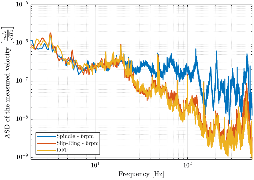
Figure 5: Comparison of the ASD of the measured velocities from the Geophone on the marble
figure;
hold on;
plot(f, sqrt(pxsp_s), 'DisplayName', 'Spindle - 6rpm');
plot(f, sqrt(pxsr_s), 'DisplayName', 'Slip-Ring - 6rpm');
plot(f, sqrt(pxof_s), 'DisplayName', 'OFF');
hold off;
set(gca, 'xscale', 'log');
set(gca, 'yscale', 'log');
xlabel('Frequency [Hz]'); ylabel('ASD of the measured velocity $\left[\frac{m/s}{\sqrt{Hz}}\right]$')
legend('Location', 'southwest');
xlim([2, 500]);
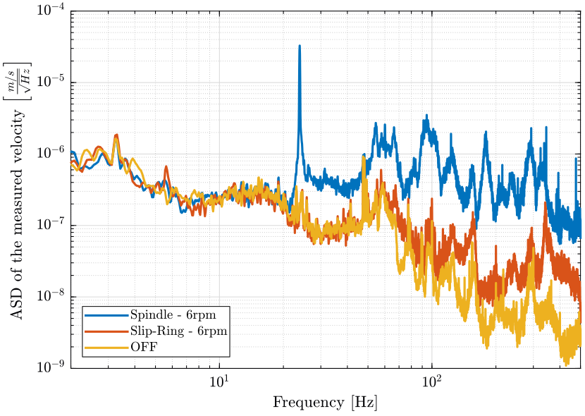
Figure 6: Comparison of the ASD of the measured velocities from the Geophone at the sample location
We load the ground motion to compare with the measurements (Fig. 7). We see that the motion is dominated by the ground motion below 20Hz.
gm = load('../ground-motion/mat/psd_gm.mat', 'f', 'psd_gv');
figure;
hold on;
plot(f, sqrt(pxsp_m), 'DisplayName', 'Spindle - 6rpm');
plot(f, sqrt(pxsr_m), 'DisplayName', 'Slip-Ring - 6rpm');
plot(f, sqrt(pxof_m), 'DisplayName', 'OFF');
plot(gm.f, sqrt(gm.psd_gv), 'k-', 'DisplayName', 'Ground Motion');
hold off;
set(gca, 'xscale', 'log');
set(gca, 'yscale', 'log');
xlabel('Frequency [Hz]'); ylabel('ASD of the measured velocity $\left[\frac{m/s}{\sqrt{Hz}}\right]$')
legend('Location', 'southwest');
xlim([2, 500]);

2.5 Relative Motion
The relative velocity between the sample and the marble is shown in Fig. 8. The velocity is integrated to have the relative displacement in Fig. 9.
Time domain: Integration to have the displacement

We compute the PSD of the relative velocity between the sample and the marble.
[pxof_r, f] = pwelch(of(:, 2)-of(:, 1), win, [], [], Fs);
[pxsr_r, ~] = pwelch(sr(:, 2)-sr(:, 1), win, [], [], Fs);
[pxsp_r, ~] = pwelch(sp(:, 2)-sp(:, 1), win, [], [], Fs);
The Power Spectral Density of the Granite Velocity, Sample velocity and relative velocity are compare in Fig. 10.
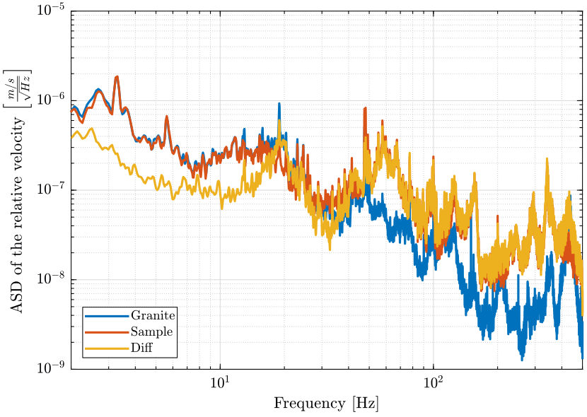
Figure 10: Comparison of the PSD of the velocity of the Sample, Granite and relative velocity (png, pdf)
Then, we display the PSD of the relative velocity for all three cases in Fig. 11.
figure;
hold on;
plot(f, sqrt(pxsp_r), 'DisplayName', 'Spindle - 6rpm');
plot(f, sqrt(pxsr_r), 'DisplayName', 'Slip-Ring - 6rpm');
plot(f, sqrt(pxof_r), 'DisplayName', 'OFF');
hold off;
set(gca, 'xscale', 'log');
set(gca, 'yscale', 'log');
xlabel('Frequency [Hz]'); ylabel('ASD of the relative velocity $\left[\frac{m/s}{\sqrt{Hz}}\right]$')
legend('Location', 'southwest');
xlim([2, 500]);
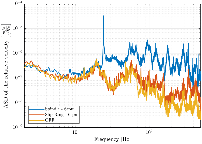
Figure 11: Comparison of the ASD of the relative velocity
The Cumulative Power Spectrum of the relative velocity is shown in Fig. 12 and in Fig. 13 (integrated in reverse direction).
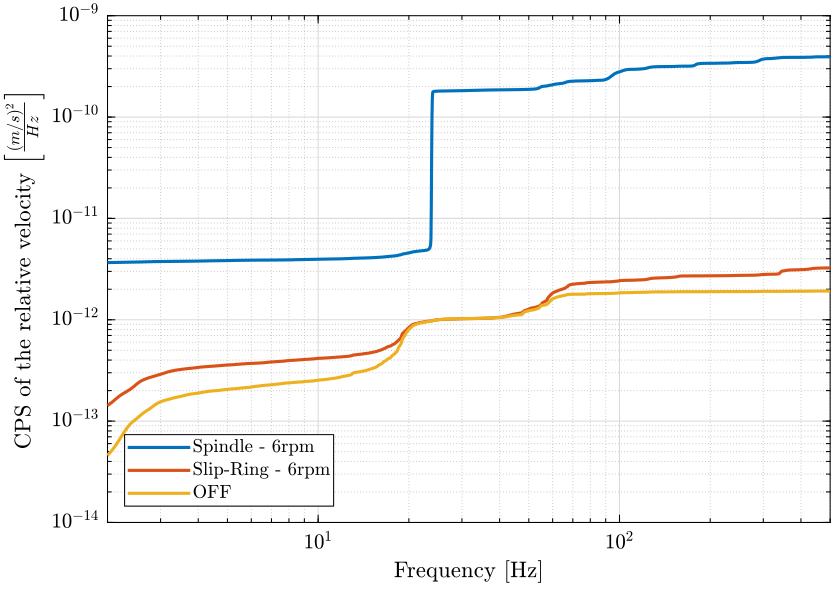

Figure 13: Cumulative Power Spectrum of the relative velocity (integrated from high to low frequencies) (png, pdf)
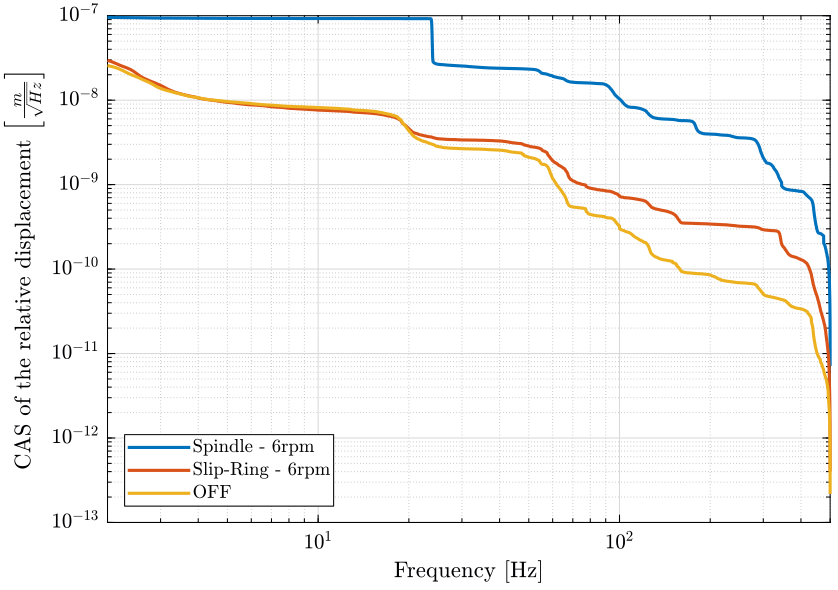
Finally, the Cumulative Amplitude Spectrum of the relative position between the hexapod and the marble is shown in Fig. 14.
figure;
hold on;
plot(f, sqrt(flip(-cumtrapz(flip(f), flip(pxsp_r./(2*pi*f).^2)))), 'DisplayName', 'Spindle - 6rpm');
plot(f, sqrt(flip(-cumtrapz(flip(f), flip(pxsr_r./(2*pi*f).^2)))), 'DisplayName', 'Slip-Ring - 6rpm');
plot(f, sqrt(flip(-cumtrapz(flip(f), flip(pxof_r./(2*pi*f).^2)))), 'DisplayName', 'OFF');
hold off;
set(gca, 'xscale', 'log'); set(gca, 'yscale', 'log');
xlabel('Frequency [Hz]'); ylabel('CAS of the relative displacement $\left[\frac{m}{\sqrt{Hz}}\right]$')
legend('Location', 'southwest');
xlim([2, 500]);
2.6 Save
The Power Spectral Density of the relative velocity and of the hexapod velocity is saved for further analysis.
save('mat/pxsp_r.mat', 'f', 'pxsp_r', 'pxsp_s');
2.7 Conclusion
The relative motion below 20Hz is dominated by another effect than the rotation of the Spindle (probably ground motion).
The Slip-Ring rotation induce almost no relative motion of the hexapod with respect to the granite (only a little above 400Hz).
The Spindle rotation induces relative motion of the hexapod with respect to the granite above 20Hz.
There is a huge peak at 24Hz on the sample vibration but not on the granite vibration
- The peak is really sharp, could this be due to magnetic effect?
- Should redo the measurement with piezo accelerometers.