Cercalo Test Bench

1. Identification
2. Plant Analysis
3. Control

1 Identification

All the files (data and Matlab scripts) are accessible here.

1.1 Excitation Data

fs = 1e4;
Ts = 1/fs;

We generate white noise with the "random number" simulink block, and we filter that noise.

Gi = (1)/(1+s/2/pi/100);

c2d(Gi, Ts, 'tustin')

c2d(Gi, Ts, 'tustin')

ans =

  0.030459 (z+1)
  --------------
    (z-0.9391)

Sample time: 0.0001 seconds
Discrete-time zero/pole/gain model.

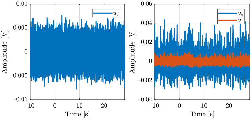
1.2 Input / Output data

The identification data is loaded

ux = load('mat/data_ux.mat', 't', 'ux', 'yx', 'yy');
uy = load('mat/data_uy.mat', 't', 'uy', 'yx', 'yy');

We remove the first seconds where the Cercalo is turned on.

i0x = 20*fs;

i0y = 10*fs;

ux.t  = ux.t( i0x:end) - ux.t(i0x);
ux.ux = ux.ux(i0x:end);
ux.yx = ux.yx(i0x:end);
ux.yy = ux.yy(i0x:end);

uy.t  = uy.t( i0y:end) - uy.t(i0x);
uy.uy = uy.uy(i0y:end);
uy.yx = uy.yx(i0y:end);
uy.yy = uy.yy(i0y:end);

ux.ux = ux.ux-mean(ux.ux);
ux.yx = ux.yx-mean(ux.yx);
ux.yy = ux.yy-mean(ux.yy);

uy.ux = uy.ux-mean(uy.ux);
uy.yx = uy.yx-mean(uy.yx);
uy.yy = uy.yy-mean(uy.yy);

Figure 1: Identification signals when exciting the \(x\) axis (png, pdf)

Figure 2: Identification signals when exciting the \(y\) axis (png, pdf)

1.3 Estimation of the Frequency Response Function Matrix

We compute an estimate of the transfer functions.

[tf_ux_yx, f] = tfestimate(ux.ux, ux.yx, hanning(ceil(1*fs)), [], [], fs);
[tf_ux_yy, ~] = tfestimate(ux.ux, ux.yy, hanning(ceil(1*fs)), [], [], fs);
[tf_uy_yx, ~] = tfestimate(uy.uy, uy.yx, hanning(ceil(1*fs)), [], [], fs);
[tf_uy_yy, ~] = tfestimate(uy.uy, uy.yy, hanning(ceil(1*fs)), [], [], fs);

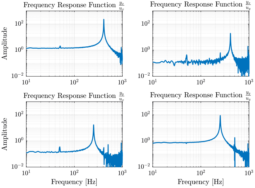
Figure 3: Frequency Response Matrix (png, pdf)

1.4 Coherence

[coh_ux_yx, f] = mscohere(ux.ux, ux.yx, hanning(ceil(1*fs)), [], [], fs);
[coh_ux_yy, ~] = mscohere(ux.ux, ux.yy, hanning(ceil(1*fs)), [], [], fs);
[coh_uy_yx, ~] = mscohere(uy.uy, uy.yx, hanning(ceil(1*fs)), [], [], fs);
[coh_uy_yy, ~] = mscohere(uy.uy, uy.yy, hanning(ceil(1*fs)), [], [], fs);

Figure 4: Coherence (png, pdf)

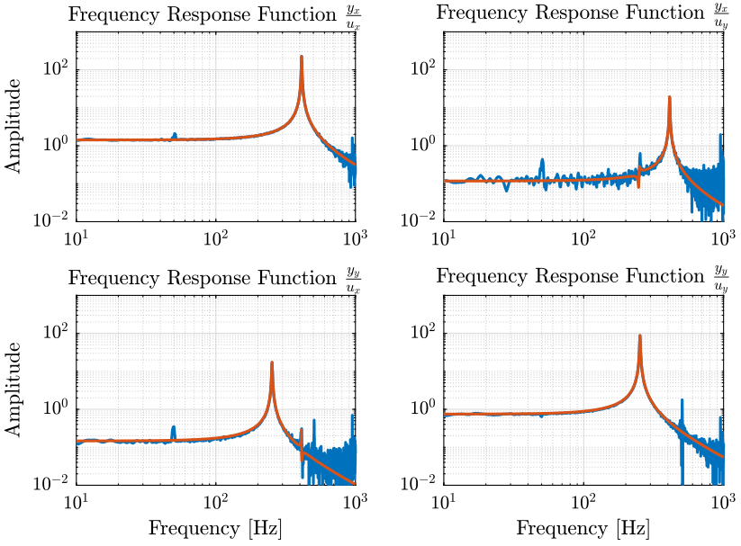
1.5 Extraction of a transfer function matrix

First we define the initial guess for the resonance frequencies and the weights associated.

freqs_res = [410, 250]; % [Hz]
freqs_res_weights = [10, 10]; % [Hz]

From the number of resonance frequency we want to fit, we define the order N of the system we want to obtain.

N = 2*length(freqs_res);

We then make an initial guess on the complex values of the poles.

xi = 0.001; % Approximate modal damping
poles = [2*pi*freqs_res*(xi + 1i), 2*pi*freqs_res*(xi - 1i)];

We then define the weight that will be used for the fitting. Basically, we want more weight around the resonance and at low frequency (below the first resonance). Also, we want more importance where we have a better coherence.

weight = ones(1, length(f));
% weight = G_coh';

% alpha = 0.1;

% for freq_i = 1:length(freqs_res)
%   weight(f>(1-alpha)*freqs_res(freq_i) & omega<(1 + alpha)*2*pi*freqs_res(freq_i)) = freqs_res_weights(freq_i);
% end

Ignore data above some frequency.

weight(f>1000) = 0;

Figure 5: Weights amplitude (png, pdf)

When we set some options for vfit3.

opts = struct();

opts.stable = 1;    % Enforce stable poles
opts.asymp = 1;     % Force D matrix to be null
opts.relax = 1;     % Use vector fitting with relaxed non-triviality constraint
opts.skip_pole = 0; % Do NOT skip pole identification
opts.skip_res = 0;  % Do NOT skip identification of residues (C,D,E)
opts.cmplx_ss = 0;  % Create real state space model with block diagonal A

opts.spy1 = 0;      % No plotting for first stage of vector fitting
opts.spy2 = 0;      % Create magnitude plot for fitting of f(s)

We define the number of iteration.

Niter = 5;

An we run the vectfit3 algorithm.

for iter = 1:Niter
  [SER_ux_yx, poles, ~, fit_ux_yx] = vectfit3(tf_ux_yx.', 1i*2*pi*f, poles, weight, opts);
end
for iter = 1:Niter
  [SER_uy_yx, poles, ~, fit_uy_yx] = vectfit3(tf_uy_yx.', 1i*2*pi*f, poles, weight, opts);
end
for iter = 1:Niter
  [SER_ux_yy, poles, ~, fit_ux_yy] = vectfit3(tf_ux_yy.', 1i*2*pi*f, poles, weight, opts);
end
for iter = 1:Niter
  [SER_uy_yy, poles, ~, fit_uy_yy] = vectfit3(tf_uy_yy.', 1i*2*pi*f, poles, weight, opts);
end

Figure 6: Transfer Function Extraction of the FRF matrix (png, pdf)

And finally, we create the identified state space model:

G_ux_yx = minreal(ss(full(SER_ux_yx.A),SER_ux_yx.B,SER_ux_yx.C,SER_ux_yx.D));
G_uy_yx = minreal(ss(full(SER_uy_yx.A),SER_uy_yx.B,SER_uy_yx.C,SER_uy_yx.D));
G_ux_yy = minreal(ss(full(SER_ux_yy.A),SER_ux_yy.B,SER_ux_yy.C,SER_ux_yy.D));
G_uy_yy = minreal(ss(full(SER_uy_yy.A),SER_uy_yy.B,SER_uy_yy.C,SER_uy_yy.D));

G = [G_ux_yx, G_uy_yx;
     G_ux_yy, G_uy_yy];

save('mat/plant.mat', 'G');