Finite Element Model with Simscape
Table of Contents
- 1. Amplified Piezoelectric Actuator - 3D elements
- 1.1. Import Mass Matrix, Stiffness Matrix, and Interface Nodes Coordinates
- 1.2. Output parameters
- 1.3. Piezoelectric parameters
- 1.4. Identification of the Dynamics
- 1.5. Comparison with Ansys
- 1.6. Force Sensor
- 1.7. Distributed Actuator
- 1.8. Distributed Actuator and Force Sensor
- 1.9. Dynamics from input voltage to displacement
- 1.10. Dynamics from input voltage to output voltage
- 1.11. Identification for a simpler model
- 2. APA300ML
- 2.1. Import Mass Matrix, Stiffness Matrix, and Interface Nodes Coordinates
- 2.2. Output parameters
- 2.3. Piezoelectric parameters
- 2.4. Identification of the APA Characteristics
- 2.5. Identification of the Dynamics
- 2.6. IFF
- 2.7. DVF
- 2.8. Identification for a simpler model
- 2.9. Identification of the stiffness properties
- 2.10. Effect of APA300ML in the flexibility of the leg
- 3. Flexible Joint
- 4. Optimal Flexible Joint
- 5. Integral Force Feedback with Amplified Piezo
- 6. Complete Strut with Encoder
1 Amplified Piezoelectric Actuator - 3D elements
The idea here is to:
- export a FEM of an amplified piezoelectric actuator from Ansys to Matlab
- import it into a Simscape model
- compare the obtained dynamics
- add 10kg mass on top of the actuator and identify the dynamics
- compare with results from Ansys where 10kg are directly added to the FEM
1.1 Import Mass Matrix, Stiffness Matrix, and Interface Nodes Coordinates
We first extract the stiffness and mass matrices.
K = extractMatrix('piezo_amplified_3d_K.txt');
M = extractMatrix('piezo_amplified_3d_M.txt');
Then, we extract the coordinates of the interface nodes.
[int_xyz, int_i, n_xyz, n_i, nodes] = extractNodes('piezo_amplified_3d.txt');
save('./mat/piezo_amplified_3d.mat', 'int_xyz', 'int_i', 'n_xyz', 'n_i', 'nodes', 'M', 'K');
1.2 Output parameters
load('./mat/piezo_amplified_3d.mat', 'int_xyz', 'int_i', 'n_xyz', 'n_i', 'nodes', 'M', 'K');
| Total number of Nodes | 168959 |
| Number of interface Nodes | 13 |
| Number of Modes | 30 |
| Size of M and K matrices | 108 |
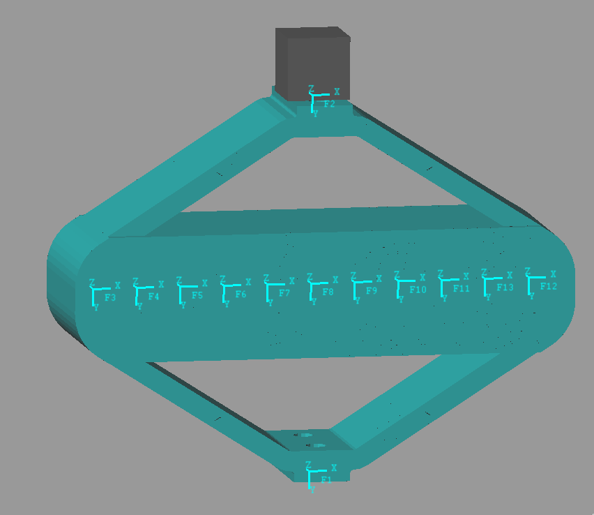
Figure 1: Interface Nodes for the Amplified Piezo Actuator
| Node i | Node Number | x [m] | y [m] | z [m] |
|---|---|---|---|---|
| 1.0 | 168947.0 | 0.0 | 0.03 | 0.0 |
| 2.0 | 168949.0 | 0.0 | -0.03 | 0.0 |
| 3.0 | 168950.0 | -0.035 | 0.0 | 0.0 |
| 4.0 | 168951.0 | -0.028 | 0.0 | 0.0 |
| 5.0 | 168952.0 | -0.021 | 0.0 | 0.0 |
| 6.0 | 168953.0 | -0.014 | 0.0 | 0.0 |
| 7.0 | 168954.0 | -0.007 | 0.0 | 0.0 |
| 8.0 | 168955.0 | 0.0 | 0.0 | 0.0 |
| 9.0 | 168956.0 | 0.007 | 0.0 | 0.0 |
| 10.0 | 168957.0 | 0.014 | 0.0 | 0.0 |
| 11.0 | 168958.0 | 0.021 | 0.0 | 0.0 |
| 12.0 | 168959.0 | 0.035 | 0.0 | 0.0 |
| 13.0 | 168960.0 | 0.028 | 0.0 | 0.0 |
| 300000000.0 | -30000.0 | 8000.0 | -200.0 | -30.0 | -60000.0 | 20000000.0 | -4000.0 | 500.0 | 8 |
| -30000.0 | 100000000.0 | 400.0 | 30.0 | 200.0 | -1 | 4000.0 | -8000000.0 | 800.0 | 7 |
| 8000.0 | 400.0 | 50000000.0 | -800000.0 | -300.0 | -40.0 | 300.0 | 100.0 | 5000000.0 | 40000.0 |
| -200.0 | 30.0 | -800000.0 | 20000.0 | 5 | 1 | -10.0 | -2 | -40000.0 | -300.0 |
| -30.0 | 200.0 | -300.0 | 5 | 40000.0 | 0.3 | -4 | -10.0 | 40.0 | 0.4 |
| -60000.0 | -1 | -40.0 | 1 | 0.3 | 3000.0 | 7000.0 | 0.8 | -1 | 0.0003 |
| 20000000.0 | 4000.0 | 300.0 | -10.0 | -4 | 7000.0 | 300000000.0 | 20000.0 | 3000.0 | 80.0 |
| -4000.0 | -8000000.0 | 100.0 | -2 | -10.0 | 0.8 | 20000.0 | 100000000.0 | -4000.0 | -100.0 |
| 500.0 | 800.0 | 5000000.0 | -40000.0 | 40.0 | -1 | 3000.0 | -4000.0 | 50000000.0 | 800000.0 |
| 8 | 7 | 40000.0 | -300.0 | 0.4 | 0.0003 | 80.0 | -100.0 | 800000.0 | 20000.0 |
| 0.03 | 2e-06 | -2e-07 | 1e-08 | 2e-08 | 0.0002 | -0.001 | 2e-07 | -8e-08 | -9e-10 |
| 2e-06 | 0.02 | -5e-07 | 7e-09 | 3e-08 | 2e-08 | -3e-07 | 0.0003 | -1e-08 | 1e-10 |
| -2e-07 | -5e-07 | 0.02 | -9e-05 | 4e-09 | -1e-08 | 2e-07 | -2e-08 | -0.0006 | -5e-06 |
| 1e-08 | 7e-09 | -9e-05 | 1e-06 | 6e-11 | 4e-10 | -1e-09 | 3e-11 | 5e-06 | 3e-08 |
| 2e-08 | 3e-08 | 4e-09 | 6e-11 | 1e-06 | 2e-10 | -2e-09 | 2e-10 | -7e-09 | -4e-11 |
| 0.0002 | 2e-08 | -1e-08 | 4e-10 | 2e-10 | 2e-06 | -2e-06 | -1e-09 | -7e-10 | -9e-12 |
| -0.001 | -3e-07 | 2e-07 | -1e-09 | -2e-09 | -2e-06 | 0.03 | -2e-06 | -1e-07 | -5e-09 |
| 2e-07 | 0.0003 | -2e-08 | 3e-11 | 2e-10 | -1e-09 | -2e-06 | 0.02 | -8e-07 | -1e-08 |
| -8e-08 | -1e-08 | -0.0006 | 5e-06 | -7e-09 | -7e-10 | -1e-07 | -8e-07 | 0.02 | 9e-05 |
| -9e-10 | 1e-10 | -5e-06 | 3e-08 | -4e-11 | -9e-12 | -5e-09 | -1e-08 | 9e-05 | 1e-06 |
Using K, M and int_xyz, we can use the Reduced Order Flexible Solid simscape block.
1.3 Piezoelectric parameters
Parameters for the APA95ML:
d33 = 3e-10; % Strain constant [m/V]
n = 80; % Number of layers per stack
eT = 1.6e-7; % Permittivity under constant stress [F/m]
sD = 2e-11; % Elastic compliance under constant electric displacement [m2/N]
ka = 235e6; % Stack stiffness [N/m]
C = 5e-6; % Stack capactiance [F]
na = 2; % Number of stacks used as actuator
ns = 1; % Number of stacks used as force sensor
The ratio of the developed force to applied voltage is \(d_{33} n k_a\) in [N/V]. We denote this constant by \(g_a\) and: \[ F_a = g_a V_a, \quad g_a = d_{33} n k_a \]
d33*(na*n)*(ka/(na + ns)) % [N/V]
3.76
From (Fleming and Leang 2014) (page 123), the relation between relative displacement and generated voltage is: \[ V_s = \frac{d_{33}}{\epsilon^T s^D n} \Delta h \] where:
- \(V_s\): measured voltage [V]
- \(d_{33}\): strain constant [m/V]
- \(\epsilon^T\): permittivity under constant stress [F/m]
- \(s^D\): elastic compliance under constant electric displacement [m^2/N]
- \(n\): number of layers
- \(\Delta h\): relative displacement [m]
1e-6*d33/(eT*sD*ns*n) % [V/um]
1.1719
1.4 Identification of the Dynamics
The flexible element is imported using the Reduced Order Flexible Solid simscape block.
To model the actuator, an Internal Force block is added between the nodes 3 and 12.
A Relative Motion Sensor block is added between the nodes 1 and 2 to measure the displacement and the amplified piezo.
One mass is fixed at one end of the piezo-electric stack actuator, the other end is fixed to the world frame.
We first set the mass to be zero.
m = 0.01;
The dynamics is identified from the applied force to the measured relative displacement.
%% Name of the Simulink File
mdl = 'piezo_amplified_3d';

%% Input/Output definition
clear io; io_i = 1;
io(io_i) = linio([mdl, '/F'], 1, 'openinput');  io_i = io_i + 1;
io(io_i) = linio([mdl, '/y'], 1, 'openoutput'); io_i = io_i + 1;

Gh = -linearize(mdl, io);
Then, we add 10Kg of mass:
m = 5;
And the dynamics is identified.
The two identified dynamics are compared in Figure 2.
%% Name of the Simulink File
mdl = 'piezo_amplified_3d';

%% Input/Output definition
clear io; io_i = 1;
io(io_i) = linio([mdl, '/F'], 1, 'openinput');  io_i = io_i + 1;
io(io_i) = linio([mdl, '/y'], 1, 'openoutput'); io_i = io_i + 1;

Ghm = -linearize(mdl, io);
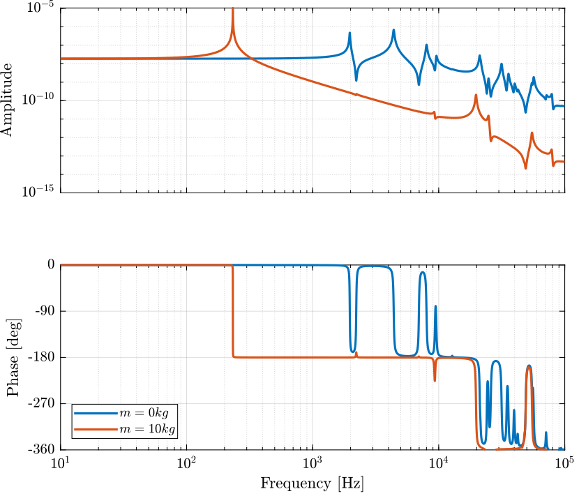
Figure 2: Dynamics from \(F\) to \(d\) without a payload and with a 10kg payload
1.5 Comparison with Ansys
Let’s import the results from an Harmonic response analysis in Ansys.
Gresp0 = readtable('FEA_HarmResponse_00kg.txt');
Gresp10 = readtable('FEA_HarmResponse_10kg.txt');
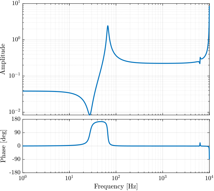
The obtained dynamics from the Simscape model and from the Ansys analysis are compare in Figure 3.
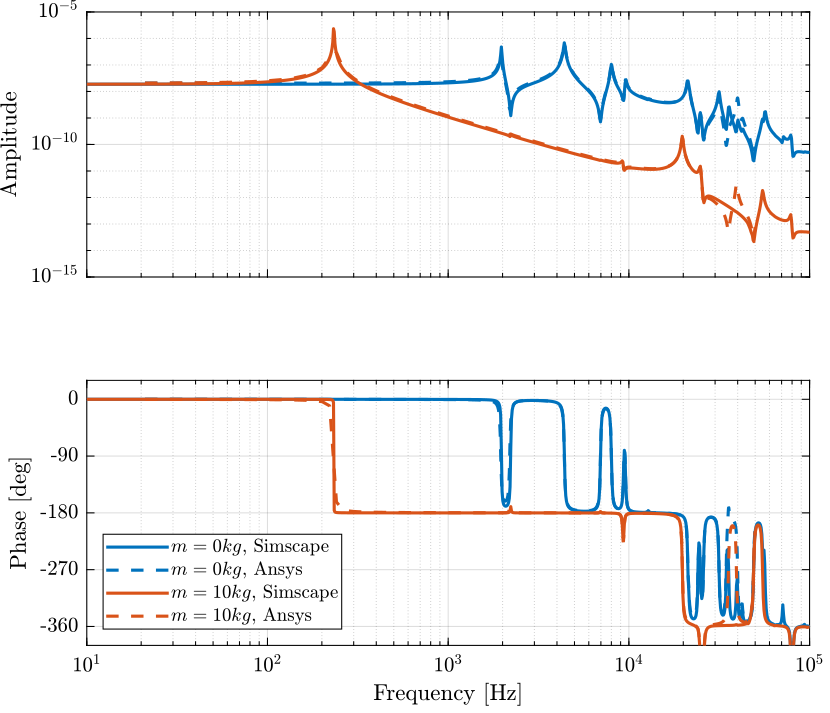
Figure 3: Comparison of the obtained dynamics using Simscape with the harmonic response analysis using Ansys
1.6 Force Sensor
The dynamics is identified from internal forces applied between nodes 3 and 11 to the relative displacement of nodes 11 and 13.
The obtained dynamics is shown in Figure 4.
m = 0;
%% Name of the Simulink File
mdl = 'piezo_amplified_3d';

%% Input/Output definition
clear io; io_i = 1;
io(io_i) = linio([mdl, '/Fa'], 1, 'openinput');  io_i = io_i + 1;
io(io_i) = linio([mdl, '/Fs'], 1, 'openoutput'); io_i = io_i + 1;

Gf = linearize(mdl, io);
m = 10;
%% Name of the Simulink File
mdl = 'piezo_amplified_3d';

%% Input/Output definition
clear io; io_i = 1;
io(io_i) = linio([mdl, '/Fa'], 1, 'openinput');  io_i = io_i + 1;
io(io_i) = linio([mdl, '/Fs'], 1, 'openoutput'); io_i = io_i + 1;

Gfm = linearize(mdl, io);

Figure 4: Dynamics from \(F\) to \(F_m\) for \(m=0\) and \(m = 10kg\)
1.7 Distributed Actuator
m = 0;
The dynamics is identified from the applied force to the measured relative displacement.
%% Name of the Simulink File
mdl = 'piezo_amplified_3d_distri';

%% Input/Output definition
clear io; io_i = 1;
io(io_i) = linio([mdl, '/F'], 1, 'openinput');  io_i = io_i + 1;
io(io_i) = linio([mdl, '/y'], 1, 'openoutput'); io_i = io_i + 1;

Gd = linearize(mdl, io);
Then, we add 10Kg of mass:
m = 10;
And the dynamics is identified.
%% Name of the Simulink File
mdl = 'piezo_amplified_3d_distri';

%% Input/Output definition
clear io; io_i = 1;
io(io_i) = linio([mdl, '/F'], 1, 'openinput');  io_i = io_i + 1;
io(io_i) = linio([mdl, '/y'], 1, 'openoutput'); io_i = io_i + 1;

Gdm = linearize(mdl, io);
1.8 Distributed Actuator and Force Sensor
m = 0;
%% Name of the Simulink File
mdl = 'piezo_amplified_3d_distri_act_sens';

%% Input/Output definition
clear io; io_i = 1;
io(io_i) = linio([mdl, '/F'], 1, 'openinput');  io_i = io_i + 1;
io(io_i) = linio([mdl, '/Fm'], 1, 'openoutput'); io_i = io_i + 1;

Gfd = linearize(mdl, io);
m = 10;
%% Name of the Simulink File
mdl = 'piezo_amplified_3d_distri_act_sens';

%% Input/Output definition
clear io; io_i = 1;
io(io_i) = linio([mdl, '/F'], 1, 'openinput');  io_i = io_i + 1;
io(io_i) = linio([mdl, '/Fm'], 1, 'openoutput'); io_i = io_i + 1;

Gfdm = linearize(mdl, io);
1.9 Dynamics from input voltage to displacement
m = 5;
And the dynamics is identified.
The two identified dynamics are compared in Figure 2.
%% Name of the Simulink File
mdl = 'piezo_amplified_3d';

%% Input/Output definition
clear io; io_i = 1;
io(io_i) = linio([mdl, '/V'], 1, 'openinput');  io_i = io_i + 1;
io(io_i) = linio([mdl, '/y'], 1, 'openoutput'); io_i = io_i + 1;

G = -linearize(mdl, io);
save('../test-bench-apa/mat/fem_model_5kg.mat', 'G')
1.10 Dynamics from input voltage to output voltage
m = 5;
%% Name of the Simulink File
mdl = 'piezo_amplified_3d';

%% Input/Output definition
clear io; io_i = 1;
io(io_i) = linio([mdl, '/Fa'], 1, 'openinput');  io_i = io_i + 1;
io(io_i) = linio([mdl, '/dL'], 1, 'openoutput'); io_i = io_i + 1;

G = -linearize(mdl, io);
1.11 Identification for a simpler model
The goal in this section is to identify the parameters of a simple APA model from the FEM. This can be useful is a lower order model is to be used for simulations.
The presented model is based on (Souleille et al. 2018).
The model represents the Amplified Piezo Actuator (APA) from Cedrat-Technologies (Figure 5). The parameters are shown in the table below.
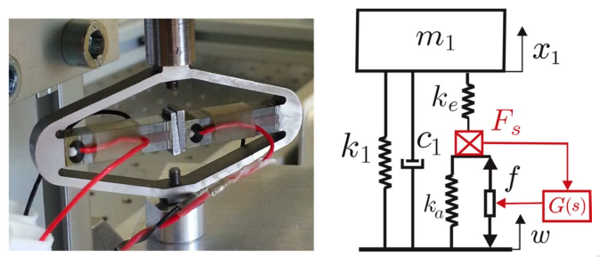
Figure 5: Picture of an APA100M from Cedrat Technologies. Simplified model of a one DoF payload mounted on such isolator
| Meaning | |
|---|---|
| \(k_e\) | Stiffness used to adjust the pole of the isolator |
| \(k_1\) | Stiffness of the metallic suspension when the stack is removed |
| \(k_a\) | Stiffness of the actuator |
| \(c_1\) | Added viscous damping |
The goal is to determine \(k_e\), \(k_a\) and \(k_1\) so that the simplified model fits the FEM model.
\[ \alpha = \frac{x_1}{f}(\omega=0) = \frac{\frac{k_e}{k_e + k_a}}{k_1 + \frac{k_e k_a}{k_e + k_a}} \] \[ \beta = \frac{x_1}{F}(\omega=0) = \frac{1}{k_1 + \frac{k_e k_a}{k_e + k_a}} \]
If we can fix \(k_a\), we can determine \(k_e\) and \(k_1\) with: \[ k_e = \frac{k_a}{\frac{\beta}{\alpha} - 1} \] \[ k_1 = \frac{1}{\beta} - \frac{k_e k_a}{k_e + k_a} \]
From the identified dynamics, compute \(\alpha\) and \(\beta\)
alpha = abs(dcgain(G('y', 'Fa')));
beta  = abs(dcgain(G('y', 'Fd')));
\(k_a\) is estimated using the following formula:
ka = 0.9/abs(dcgain(G('y', 'Fa')));
The factor can be adjusted to better match the curves.
Then \(k_e\) and \(k_1\) are computed.
ke = ka/(beta/alpha - 1);
k1 = 1/beta - ke*ka/(ke + ka);
| Value [N/um] | |
|---|---|
| ka | 54.9 |
| ke | 25.1 |
| k1 | 4.3 |
The damping in the system is adjusted to match the FEM model if necessary.
c1 = 1e2;
Analytical model of the simpler system:
Ga = 1/(m*s^2 + k1 + c1*s + ke*ka/(ke + ka)) * ...
     [ 1 ,              k1 + c1*s + ke*ka/(ke + ka)  , ke/(ke + ka) ;
      -ke*ka/(ke + ka), ke*ka/(ke + ka)*m*s^2 ,       -ke/(ke + ka)*(m*s^2 + c1*s + k1)];

Ga.InputName = {'Fd', 'w', 'Fa'};
Ga.OutputName = {'y', 'Fs'};
Adjust the DC gain for the force sensor:
F_gain = dcgain(G('Fs', 'Fd'))/dcgain(Ga('Fs', 'Fd'));

Figure 6: Comparison of the Dynamics between the FEM model and the simplified one
We save the parameters of the simplified model for the APA95ML:
save('./mat/APA95ML_simplified_model.mat', 'ka', 'ke', 'k1', 'c1', 'F_gain');
2 APA300ML
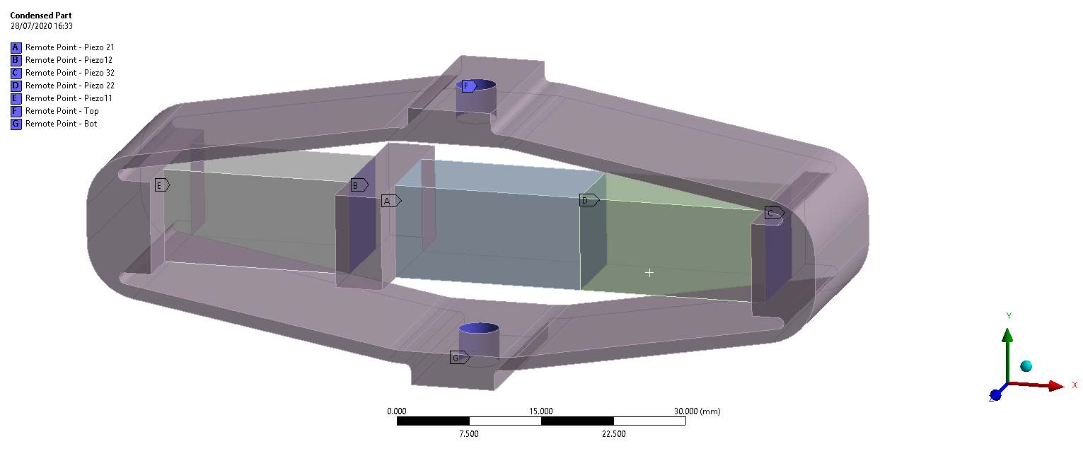
Figure 7: Ansys FEM of the APA300ML
2.1 Import Mass Matrix, Stiffness Matrix, and Interface Nodes Coordinates
We first extract the stiffness and mass matrices.
K = readmatrix('mat_K.CSV');
M = readmatrix('mat_M.CSV');
Then, we extract the coordinates of the interface nodes.
[int_xyz, int_i, n_xyz, n_i, nodes] = extractNodes('out_nodes_3D.txt');
save('./mat/APA300ML.mat', 'int_xyz', 'int_i', 'n_xyz', 'n_i', 'nodes', 'M', 'K');
2.2 Output parameters
load('./mat/APA300ML.mat', 'int_xyz', 'int_i', 'n_xyz', 'n_i', 'nodes', 'M', 'K');
| Total number of Nodes | 7 |
| Number of interface Nodes | 7 |
| Number of Modes | 120 |
| Size of M and K matrices | 162 |
| Node i | Node Number | x [m] | y [m] | z [m] |
|---|---|---|---|---|
| 1.0 | 697783.0 | 0.0 | 0.0 | -0.015 |
| 2.0 | 697784.0 | 0.0 | 0.0 | 0.015 |
| 3.0 | 697785.0 | -0.0325 | 0.0 | 0.0 |
| 4.0 | 697786.0 | -0.0125 | 0.0 | 0.0 |
| 5.0 | 697787.0 | -0.0075 | 0.0 | 0.0 |
| 6.0 | 697788.0 | 0.0125 | 0.0 | 0.0 |
| 7.0 | 697789.0 | 0.0325 | 0.0 | 0.0 |
| 200000000.0 | 30000.0 | -20000.0 | -70.0 | 300000.0 | 40.0 | 10000000.0 | 10000.0 | -6000.0 | 30.0 |
| 30000.0 | 30000000.0 | 2000.0 | -200000.0 | 60.0 | -10.0 | 4000.0 | 2000000.0 | -500.0 | 9000.0 |
| -20000.0 | 2000.0 | 7000000.0 | -10.0 | -30.0 | 10.0 | 6000.0 | 900.0 | -500000.0 | 3 |
| -70.0 | -200000.0 | -10.0 | 1000.0 | -0.1 | 0.08 | -20.0 | -9000.0 | 3 | -30.0 |
| 300000.0 | 60.0 | -30.0 | -0.1 | 900.0 | 0.1 | 30000.0 | 20.0 | -10.0 | 0.06 |
| 40.0 | -10.0 | 10.0 | 0.08 | 0.1 | 10000.0 | 20.0 | 9 | -5 | 0.03 |
| 10000000.0 | 4000.0 | 6000.0 | -20.0 | 30000.0 | 20.0 | 200000000.0 | 10000.0 | 9000.0 | 50.0 |
| 10000.0 | 2000000.0 | 900.0 | -9000.0 | 20.0 | 9 | 10000.0 | 30000000.0 | -500.0 | 200000.0 |
| -6000.0 | -500.0 | -500000.0 | 3 | -10.0 | -5 | 9000.0 | -500.0 | 7000000.0 | -2 |
| 30.0 | 9000.0 | 3 | -30.0 | 0.06 | 0.03 | 50.0 | 200000.0 | -2 | 1000.0 |
| 0.01 | -2e-06 | 1e-06 | 6e-09 | 5e-05 | -5e-09 | -0.0005 | -7e-07 | 6e-07 | -3e-09 |
| -2e-06 | 0.01 | 8e-07 | -2e-05 | -8e-09 | 2e-09 | -9e-07 | -0.0002 | 1e-08 | -9e-07 |
| 1e-06 | 8e-07 | 0.009 | 5e-10 | 1e-09 | -1e-09 | -5e-07 | 3e-08 | 6e-05 | 1e-10 |
| 6e-09 | -2e-05 | 5e-10 | 3e-07 | 2e-11 | -3e-12 | 3e-09 | 9e-07 | -4e-10 | 3e-09 |
| 5e-05 | -8e-09 | 1e-09 | 2e-11 | 6e-07 | -4e-11 | -1e-06 | -2e-09 | 1e-09 | -8e-12 |
| -5e-09 | 2e-09 | -1e-09 | -3e-12 | -4e-11 | 1e-07 | -2e-09 | -1e-09 | -4e-10 | -5e-12 |
| -0.0005 | -9e-07 | -5e-07 | 3e-09 | -1e-06 | -2e-09 | 0.01 | 1e-07 | -3e-07 | -2e-08 |
| -7e-07 | -0.0002 | 3e-08 | 9e-07 | -2e-09 | -1e-09 | 1e-07 | 0.01 | -4e-07 | 2e-05 |
| 6e-07 | 1e-08 | 6e-05 | -4e-10 | 1e-09 | -4e-10 | -3e-07 | -4e-07 | 0.009 | -2e-10 |
| -3e-09 | -9e-07 | 1e-10 | 3e-09 | -8e-12 | -5e-12 | -2e-08 | 2e-05 | -2e-10 | 3e-07 |
Using K, M and int_xyz, we can use the Reduced Order Flexible Solid simscape block.
2.3 Piezoelectric parameters
Parameters for the APA300ML:
d33 = 3e-10; % Strain constant [m/V]
n = 80; % Number of layers per stack
eT = 1.6e-8; % Permittivity under constant stress [F/m]
sD = 2e-11; % Elastic compliance under constant electric displacement [m2/N]
ka = 235e6; % Stack stiffness [N/m]
C = 5e-6; % Stack capactiance [F]
na = 2; % Number of stacks used as actuator
ns = 1; % Number of stacks used as force sensor
The ratio of the developed force to applied voltage is \(d_{33} n k_a\) in [N/V]. We denote this constant by \(g_a\) and: \[ F_a = g_a V_a, \quad g_a = d_{33} n k_a \]
d33*(na*n)*(ka/(na + ns)) % [N/V]
3.76
From (Fleming and Leang 2014) (page 123), the relation between relative displacement and generated voltage is: \[ V_s = \frac{d_{33}}{\epsilon^T s^D n} \Delta h \] where:
- \(V_s\): measured voltage [V]
- \(d_{33}\): strain constant [m/V]
- \(\epsilon^T\): permittivity under constant stress [F/m]
- \(s^D\): elastic compliance under constant electric displacement [m^2/N]
- \(n\): number of layers
- \(\Delta h\): relative displacement [m]
1e-6*d33/(eT*sD*ns*n) % [V/um]
11.719
2.4 Identification of the APA Characteristics
2.4.1 Stiffness
The transfer function from vertical external force to the relative vertical displacement is identified.
The inverse of its DC gain is the axial stiffness of the APA:
1e-6/dcgain(G) % [N/um]
1.753
The specified stiffness in the datasheet is \(k = 1.8\, [N/\mu m]\).
2.4.2 Resonance Frequency
The resonance frequency is specified to be between 650Hz and 840Hz. This is also the case for the FEM model (Figure 8).
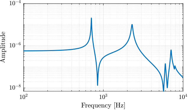
Figure 8: First resonance is around 800Hz
2.4.3 Amplification factor
The amplification factor is the ratio of the axial displacement to the stack displacement.
The ratio of the two displacement is computed from the FEM model.
abs(dcgain(G(1,1))./dcgain(G(2,1)))
5.0749
If we take the ratio of the piezo height and length (approximation of the amplification factor):
75/15
5
2.4.4 Stroke
Estimation of the actuator stroke: \[ \Delta H = A n \Delta L \] with:
- \(\Delta H\) Axial Stroke of the APA
- \(A\) Amplification factor (5 for the APA300ML)
- \(n\) Number of stack used
- \(\Delta L\) Stroke of the stack (0.1% of its length)
1e6 * 5 * 3 * 20e-3 * 0.1e-2
300
This is exactly the specified stroke in the data-sheet.
2.5 Identification of the Dynamics
The flexible element is imported using the Reduced Order Flexible Solid simscape block.
To model the actuator, an Internal Force block is added between the nodes 3 and 12.
A Relative Motion Sensor block is added between the nodes 1 and 2 to measure the displacement and the amplified piezo.
One mass is fixed at one end of the piezo-electric stack actuator, the other end is fixed to the world frame.
We first set the mass to be zero. The dynamics is identified from the applied force to the measured relative displacement. The same dynamics is identified for a payload mass of 10Kg.
m = 10;
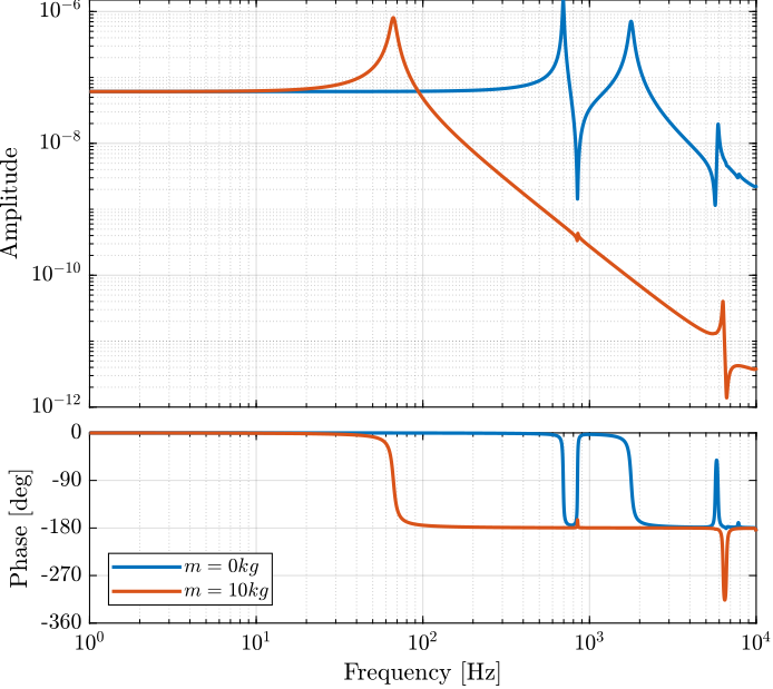
Figure 9: Transfer function from forces applied by the stack to the axial displacement of the APA
2.6 IFF
2.7 DVF
2.8 Identification for a simpler model
The goal in this section is to identify the parameters of a simple APA model from the FEM. This can be useful is a lower order model is to be used for simulations.
The presented model is based on (Souleille et al. 2018).
The model represents the Amplified Piezo Actuator (APA) from Cedrat-Technologies (Figure 5). The parameters are shown in the table below.
Figure 14: Picture of an APA100M from Cedrat Technologies. Simplified model of a one DoF payload mounted on such isolator
| Meaning | |
|---|---|
| \(k_e\) | Stiffness used to adjust the pole of the isolator |
| \(k_1\) | Stiffness of the metallic suspension when the stack is removed |
| \(k_a\) | Stiffness of the actuator |
| \(c_1\) | Added viscous damping |
The goal is to determine \(k_e\), \(k_a\) and \(k_1\) so that the simplified model fits the FEM model.
\[ \alpha = \frac{x_1}{f}(\omega=0) = \frac{\frac{k_e}{k_e + k_a}}{k_1 + \frac{k_e k_a}{k_e + k_a}} \] \[ \beta = \frac{x_1}{F}(\omega=0) = \frac{1}{k_1 + \frac{k_e k_a}{k_e + k_a}} \]
If we can fix \(k_a\), we can determine \(k_e\) and \(k_1\) with: \[ k_e = \frac{k_a}{\frac{\beta}{\alpha} - 1} \] \[ k_1 = \frac{1}{\beta} - \frac{k_e k_a}{k_e + k_a} \]
From the identified dynamics, compute \(\alpha\) and \(\beta\)
alpha = abs(dcgain(G('y', 'Fa')));
beta  = abs(dcgain(G('y', 'Fd')));
\(k_a\) is estimated using the following formula:
ka = 0.8/abs(dcgain(G('y', 'Fa')));
The factor can be adjusted to better match the curves.
Then \(k_e\) and \(k_1\) are computed.
ke = ka/(beta/alpha - 1);
k1 = 1/beta - ke*ka/(ke + ka);
| Value [N/um] | |
|---|---|
| ka | 40.5 |
| ke | 1.5 |
| k1 | 0.4 |
The damping in the system is adjusted to match the FEM model if necessary.
c1 = 1e2;
Analytical model of the simpler system:
Ga = 1/(m*s^2 + k1 + c1*s + ke*ka/(ke + ka)) * ...
     [ 1 ,              k1 + c1*s + ke*ka/(ke + ka)  , ke/(ke + ka) ;
      -ke*ka/(ke + ka), ke*ka/(ke + ka)*m*s^2 ,       -ke/(ke + ka)*(m*s^2 + c1*s + k1)];

Ga.InputName = {'Fd', 'w', 'Fa'};
Ga.OutputName = {'y', 'Fs'};
Adjust the DC gain for the force sensor:
F_gain = dcgain(G('Fs', 'Fd'))/dcgain(Ga('Fs', 'Fd'));
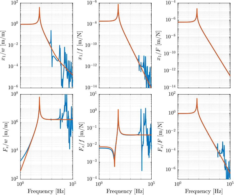
Figure 15: Comparison of the Dynamics between the FEM model and the simplified one
We now compare the FEM model with the simplified simscape model.

Figure 16: Comparison of the Dynamics between the FEM model and the simplified simscape model
We save the parameters of the simplified model for the APA300ML:
save('./mat/APA300ML_simplified_model.mat', 'ka', 'ke', 'k1', 'c1', 'F_gain');
2.9 Identification of the stiffness properties
2.9.1 APA Alone
| Caracteristics | Value |
|---|---|
| Kx [N/um] | 0.8 |
| Ky [N/um] | 1.6 |
| Kz [N/um] | 1.8 |
| Rx [Nm/rad] | 71.4 |
| Ry [Nm/rad] | 148.2 |
| Rz [Nm/rad] | 4241.8 |
2.9.2 See how the global stiffness is changing with the flexible joints
flex = load('./mat/flexor_ID16.mat', 'int_xyz', 'int_i', 'n_xyz', 'n_i', 'nodes', 'M', 'K');
| Caracteristic | Value |
|---|---|
| Kx [N/um] | 0.0 |
| Ky [N/um] | 0.0 |
| Kz [N/um] | 1.8 |
| Rx [Nm/rad] | 722.9 |
| Ry [Nm/rad] | 129.6 |
| Rz [Nm/rad] | 115.3 |
freqs = logspace(-2, 5, 1000);

figure;
hold on;
plot(freqs, abs(squeeze(freqresp(G(2,2), freqs, 'Hz'))), '-', 'DisplayName', 'APA');
plot(freqs, abs(squeeze(freqresp(Gf(2,2), freqs, 'Hz'))), '-', 'DisplayName', 'Flex');
hold off;
set(gca, 'XScale', 'log'); set(gca, 'YScale', 'log');
xlabel('Frequency [Hz]'); ylabel('Amplitude [m/N]');
hold off;
legend('location', 'northeast');
freqs = logspace(-2, 5, 1000);

figure;
hold on;
plot(freqs, abs(squeeze(freqresp(G(3,3), freqs, 'Hz'))), '-', 'DisplayName', 'APA');
plot(freqs, abs(squeeze(freqresp(Gf(3,3), freqs, 'Hz'))), '-', 'DisplayName', 'Flex');
hold off;
set(gca, 'XScale', 'log'); set(gca, 'YScale', 'log');
xlabel('Frequency [Hz]'); ylabel('Amplitude [m/N]');
hold off;
legend('location', 'northeast');
2.10 Effect of APA300ML in the flexibility of the leg
| Caracteristic | Rigid APA | Flexible APA |
|---|---|---|
| Kx [N/um] | 0.018 | 0.019 |
| Ky [N/um] | 0.018 | 0.018 |
| Kz [N/um] | 60.0 | 2.647 |
| Rx [Nm/rad] | 16.705 | 557.682 |
| Ry [Nm/rad] | 16.535 | 185.939 |
| Rz [Nm/rad] | 118.0 | 114.803 |
3 Flexible Joint
The studied flexor is shown in Figure 17.
The stiffness and mass matrices representing the dynamics of the flexor are exported from a FEM. It is then imported into Simscape.
A simplified model of the flexor is then developped.
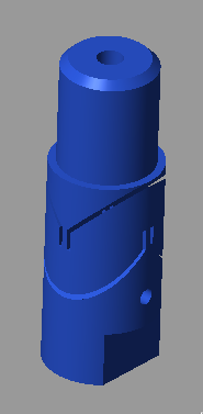
Figure 17: Flexor studied
3.1 Import Mass Matrix, Stiffness Matrix, and Interface Nodes Coordinates
We first extract the stiffness and mass matrices.
K = extractMatrix('mat_K_6modes_2MDoF.matrix');
M = extractMatrix('mat_M_6modes_2MDoF.matrix');
Then, we extract the coordinates of the interface nodes.
[int_xyz, int_i, n_xyz, n_i, nodes] = extractNodes('out_nodes_3D.txt');
save('./mat/flexor_ID16.mat', 'int_xyz', 'int_i', 'n_xyz', 'n_i', 'nodes', 'M', 'K');
3.2 Output parameters
load('./mat/flexor_ID16.mat', 'int_xyz', 'int_i', 'n_xyz', 'n_i', 'nodes', 'M', 'K');
| Total number of Nodes | 2 |
| Number of interface Nodes | 2 |
| Number of Modes | 6 |
| Size of M and K matrices | 18 |
| Node i | Node Number | x [m] | y [m] | z [m] |
|---|---|---|---|---|
| 1.0 | 181278.0 | 0.0 | 0.0 | 0.0 |
| 2.0 | 181279.0 | 0.0 | 0.0 | -0.0 |
| 11200000.0 | 195.0 | 2220.0 | -0.719 | -265.0 | 1.59 | -11200000.0 | -213.0 | -2220.0 | 0.147 |
| 195.0 | 11400000.0 | 1290.0 | -148.0 | -0.188 | 2.41 | -212.0 | -11400000.0 | -1290.0 | 148.0 |
| 2220.0 | 1290.0 | 119000000.0 | 1.31 | 1.49 | 1.79 | -2220.0 | -1290.0 | -119000000.0 | -1.31 |
| -0.719 | -148.0 | 1.31 | 33.0 | 0.000488 | -0.000977 | 0.141 | 148.0 | -1.31 | -33.0 |
| -265.0 | -0.188 | 1.49 | 0.000488 | 33.0 | 0.00293 | 266.0 | 0.154 | -1.49 | 0.00026 |
| 1.59 | 2.41 | 1.79 | -0.000977 | 0.00293 | 236.0 | -1.32 | -2.55 | -1.79 | 0.000379 |
| -11200000.0 | -212.0 | -2220.0 | 0.141 | 266.0 | -1.32 | 11400000.0 | 24600.0 | 1640.0 | 120.0 |
| -213.0 | -11400000.0 | -1290.0 | 148.0 | 0.154 | -2.55 | 24600.0 | 11400000.0 | 1290.0 | -72.0 |
| -2220.0 | -1290.0 | -119000000.0 | -1.31 | -1.49 | -1.79 | 1640.0 | 1290.0 | 119000000.0 | 1.32 |
| 0.147 | 148.0 | -1.31 | -33.0 | 0.00026 | 0.000379 | 120.0 | -72.0 | 1.32 | 34.7 |
| 0.02 | 1e-09 | -4e-08 | -1e-10 | 0.0002 | -3e-11 | 0.004 | 5e-08 | 7e-08 | 1e-10 |
| 1e-09 | 0.02 | -3e-07 | -0.0002 | -1e-10 | -2e-09 | 2e-08 | 0.004 | 3e-07 | 1e-05 |
| -4e-08 | -3e-07 | 0.02 | 7e-10 | -2e-09 | 1e-09 | 3e-07 | 7e-08 | 0.003 | 1e-09 |
| -1e-10 | -0.0002 | 7e-10 | 4e-06 | -1e-12 | -6e-13 | 2e-10 | -7e-06 | -8e-10 | -1e-09 |
| 0.0002 | -1e-10 | -2e-09 | -1e-12 | 3e-06 | 2e-13 | 9e-06 | 4e-11 | 2e-09 | -3e-13 |
| -3e-11 | -2e-09 | 1e-09 | -6e-13 | 2e-13 | 4e-07 | 8e-11 | 9e-10 | -1e-09 | 2e-12 |
| 0.004 | 2e-08 | 3e-07 | 2e-10 | 9e-06 | 8e-11 | 0.02 | -7e-08 | -3e-07 | -2e-10 |
| 5e-08 | 0.004 | 7e-08 | -7e-06 | 4e-11 | 9e-10 | -7e-08 | 0.01 | -4e-08 | 0.0002 |
| 7e-08 | 3e-07 | 0.003 | -8e-10 | 2e-09 | -1e-09 | -3e-07 | -4e-08 | 0.02 | -1e-09 |
| 1e-10 | 1e-05 | 1e-09 | -1e-09 | -3e-13 | 2e-12 | -2e-10 | 0.0002 | -1e-09 | 2e-06 |
Using K, M and int_xyz, we can use the Reduced Order Flexible Solid simscape block.
3.3 Flexible Joint Characteristics
The most important parameters of the flexible joint can be directly estimated from the stiffness matrix.
| Caracteristic | Value | Estimation by Francois |
|---|---|---|
| Axial Stiffness [N/um] | 119 | 60 |
| Shear Stiffness [N/um] | 11 | 0 |
| Bending Stiffness [Nm/rad] | 33 | 15 |
| Bending Stiffness [Nm/rad] | 33 | 15 |
| Torsion Stiffness [Nm/rad] | 236 | 20 |
3.4 Identification of the parameters using Simscape
The flexor is now imported into Simscape and its parameters are estimated using an identification.
The dynamics is identified from the applied force/torque to the measured displacement/rotation of the flexor. And we find the same parameters as the one estimated from the Stiffness matrix.
| Caracteristic | Value | Identification |
|---|---|---|
| Axial Stiffness Dz [N/um] | 119 | 119 |
| Bending Stiffness Rx [Nm/rad] | 33 | 34 |
| Bending Stiffness Ry [Nm/rad] | 33 | 126 |
| Torsion Stiffness Rz [Nm/rad] | 236 | 238 |
3.5 Simpler Model
Let’s now model the flexible joint with a “perfect” Bushing joint as shown in Figure 18.
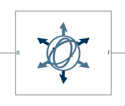
Figure 18: Bushing Joint used to model the flexible joint
The parameters of the Bushing joint (stiffnesses) are estimated from the Stiffness matrix that was computed from the FEM.
Kx = K(1,1); % [N/m]
Ky = K(2,2); % [N/m]
Kz = K(3,3); % [N/m]
Krx = K(4,4); % [Nm/rad]
Kry = K(5,5); % [Nm/rad]
Krz =  K(6,6); % [Nm/rad]
The dynamics from the applied force/torque to the measured displacement/rotation of the flexor is identified again for this simpler model. The two obtained dynamics are compared in Figure
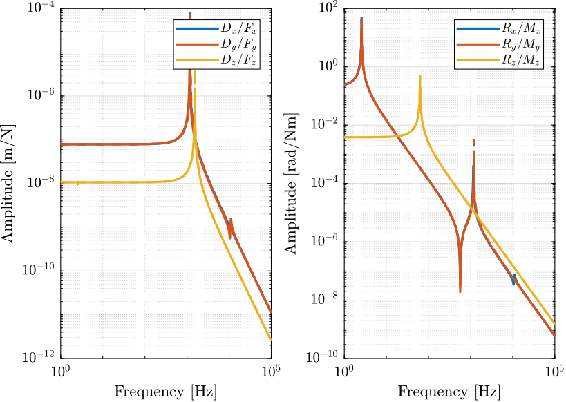
Figure 19: Comparison of the Joint compliance between the FEM model and the simpler model
4 Optimal Flexible Joint

Figure 20: Flexor studied
4.1 Import Mass Matrix, Stiffness Matrix, and Interface Nodes Coordinates
We first extract the stiffness and mass matrices.
K = readmatrix('mat_K.CSV');
M = readmatrix('mat_M.CSV');
Then, we extract the coordinates of the interface nodes.
[int_xyz, int_i, n_xyz, n_i, nodes] = extractNodes('out_nodes_3D.txt');
save('./mat/flexor_025.mat', 'int_xyz', 'int_i', 'n_xyz', 'n_i', 'nodes', 'M', 'K');
4.2 Output parameters
load('./mat/flexor_025.mat', 'int_xyz', 'int_i', 'n_xyz', 'n_i', 'nodes', 'M', 'K');
| Total number of Nodes | 2 |
| Number of interface Nodes | 2 |
| Number of Modes | 6 |
| Size of M and K matrices | 18 |
| Node i | Node Number | x [m] | y [m] | z [m] |
|---|---|---|---|---|
| 1.0 | 528875.0 | 0.0 | 0.0 | 0.0 |
| 2.0 | 528876.0 | 0.0 | 0.0 | -0.0 |
| 12700000.0 | -18.5 | -26.8 | 0.00162 | -4.63 | 64.0 | -12700000.0 | 18.3 | 26.7 | 0.00234 |
| -18.5 | 12700000.0 | -499.0 | -132.0 | 0.00414 | -0.495 | 18.4 | -12700000.0 | 499.0 | 132.0 |
| -26.8 | -499.0 | 94000000.0 | -470.0 | 0.00771 | -0.855 | 26.8 | 498.0 | -94000000.0 | 470.0 |
| 0.00162 | -132.0 | -470.0 | 4.83 | 2.61e-07 | 0.000123 | -0.00163 | 132.0 | 470.0 | -4.83 |
| -4.63 | 0.00414 | 0.00771 | 2.61e-07 | 4.83 | 4.43e-05 | 4.63 | -0.00413 | -0.00772 | -4.3e-07 |
| 64.0 | -0.495 | -0.855 | 0.000123 | 4.43e-05 | 260.0 | -64.0 | 0.495 | 0.855 | -0.000124 |
| -12700000.0 | 18.4 | 26.8 | -0.00163 | 4.63 | -64.0 | 12700000.0 | -18.2 | -26.7 | -0.00234 |
| 18.3 | -12700000.0 | 498.0 | 132.0 | -0.00413 | 0.495 | -18.2 | 12700000.0 | -498.0 | -132.0 |
| 26.7 | 499.0 | -94000000.0 | 470.0 | -0.00772 | 0.855 | -26.7 | -498.0 | 94000000.0 | -470.0 |
| 0.00234 | 132.0 | 470.0 | -4.83 | -4.3e-07 | -0.000124 | -0.00234 | -132.0 | -470.0 | 4.83 |
| 0.006 | 8e-09 | -2e-08 | -1e-10 | 3e-05 | 3e-08 | 0.003 | -3e-09 | 9e-09 | 2e-12 |
| 8e-09 | 0.02 | 1e-07 | -3e-05 | 1e-11 | 6e-10 | 1e-08 | 0.003 | -5e-08 | 3e-09 |
| -2e-08 | 1e-07 | 0.01 | -6e-08 | -6e-11 | -8e-12 | -1e-07 | 1e-08 | 0.003 | -1e-08 |
| -1e-10 | -3e-05 | -6e-08 | 1e-06 | 7e-14 | 6e-13 | 1e-10 | 1e-06 | -1e-08 | 3e-10 |
| 3e-05 | 1e-11 | -6e-11 | 7e-14 | 2e-07 | 1e-10 | 3e-08 | -7e-12 | 6e-11 | -6e-16 |
| 3e-08 | 6e-10 | -8e-12 | 6e-13 | 1e-10 | 5e-07 | 1e-08 | -5e-10 | -1e-11 | 1e-13 |
| 0.003 | 1e-08 | -1e-07 | 1e-10 | 3e-08 | 1e-08 | 0.02 | -2e-08 | 1e-07 | -4e-12 |
| -3e-09 | 0.003 | 1e-08 | 1e-06 | -7e-12 | -5e-10 | -2e-08 | 0.006 | -8e-08 | 3e-05 |
| 9e-09 | -5e-08 | 0.003 | -1e-08 | 6e-11 | -1e-11 | 1e-07 | -8e-08 | 0.01 | -6e-08 |
| 2e-12 | 3e-09 | -1e-08 | 3e-10 | -6e-16 | 1e-13 | -4e-12 | 3e-05 | -6e-08 | 2e-07 |
Using K, M and int_xyz, we can use the Reduced Order Flexible Solid simscape block.
4.3 Flexible Joint Characteristics
The most important parameters of the flexible joint can be directly estimated from the stiffness matrix.
| Caracteristic | Value |
|---|---|
| Axial Stiffness [N/um] | 94.0 |
| Shear Stiffness [N/um] | 12.7 |
| Bending Stiffness [Nm/rad] | 4.8 |
| Bending Stiffness [Nm/rad] | 4.8 |
| Torsion Stiffness [Nm/rad] | 260.2 |
4.4 Identification of the parameters using Simscape
The flexor is now imported into Simscape and its parameters are estimated using an identification.
The dynamics is identified from the applied force/torque to the measured displacement/rotation of the flexor. And we find the same parameters as the one estimated from the Stiffness matrix.
| Caracteristic | Value | Identification |
|---|---|---|
| Axial Stiffness Dz [N/um] | 94.0 | 93.9 |
| Bending Stiffness Rx [Nm/rad] | 4.8 | 4.8 |
| Bending Stiffness Ry [Nm/rad] | 4.8 | 4.8 |
| Torsion Stiffness Rz [Nm/rad] | 260.2 | 260.2 |
4.5 Simpler Model
Let’s now model the flexible joint with a “perfect” Bushing joint as shown in Figure 18.
Figure 21: Bushing Joint used to model the flexible joint
The parameters of the Bushing joint (stiffnesses) are estimated from the Stiffness matrix that was computed from the FEM.
Kx = K(1,1); % [N/m]
Ky = K(2,2); % [N/m]
Kz = K(3,3); % [N/m]
Krx = K(4,4); % [Nm/rad]
Kry = K(5,5); % [Nm/rad]
Krz =  K(6,6); % [Nm/rad]
The dynamics from the applied force/torque to the measured displacement/rotation of the flexor is identified again for this simpler model. The two obtained dynamics are compared in Figure
Figure 22: Comparison of the Joint compliance between the FEM model and the simpler model
5 Integral Force Feedback with Amplified Piezo
In this section, we try to replicate the results obtained in (Souleille et al. 2018).
5.1 Import Mass Matrix, Stiffness Matrix, and Interface Nodes Coordinates
We first extract the stiffness and mass matrices.
K = extractMatrix('piezo_amplified_IFF_K.txt');
M = extractMatrix('piezo_amplified_IFF_M.txt');
Then, we extract the coordinates of the interface nodes.
[int_xyz, int_i, n_xyz, n_i, nodes] = extractNodes('piezo_amplified_IFF.txt');
5.2 IFF Plant
The transfer function from the force actuator to the force sensor is identified and shown in Figure 23.
Kiff = tf(0);
m = 0;
%% Name of the Simulink File
mdl = 'piezo_amplified_IFF';

%% Input/Output definition
clear io; io_i = 1;
io(io_i) = linio([mdl, '/Kiff'], 1, 'openinput');  io_i = io_i + 1;
io(io_i) = linio([mdl, '/G'],    1, 'openoutput'); io_i = io_i + 1;

Gf = linearize(mdl, io);
m = 10;
Gfm = linearize(mdl, io);
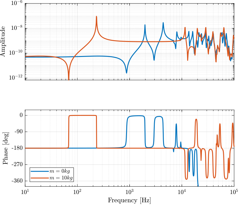
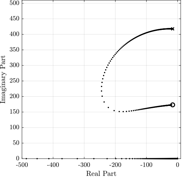
Figure 23: IFF Plant
5.3 IFF controller
The controller is defined and the loop gain is shown in Figure 24.
Kiff = -1e12/s;
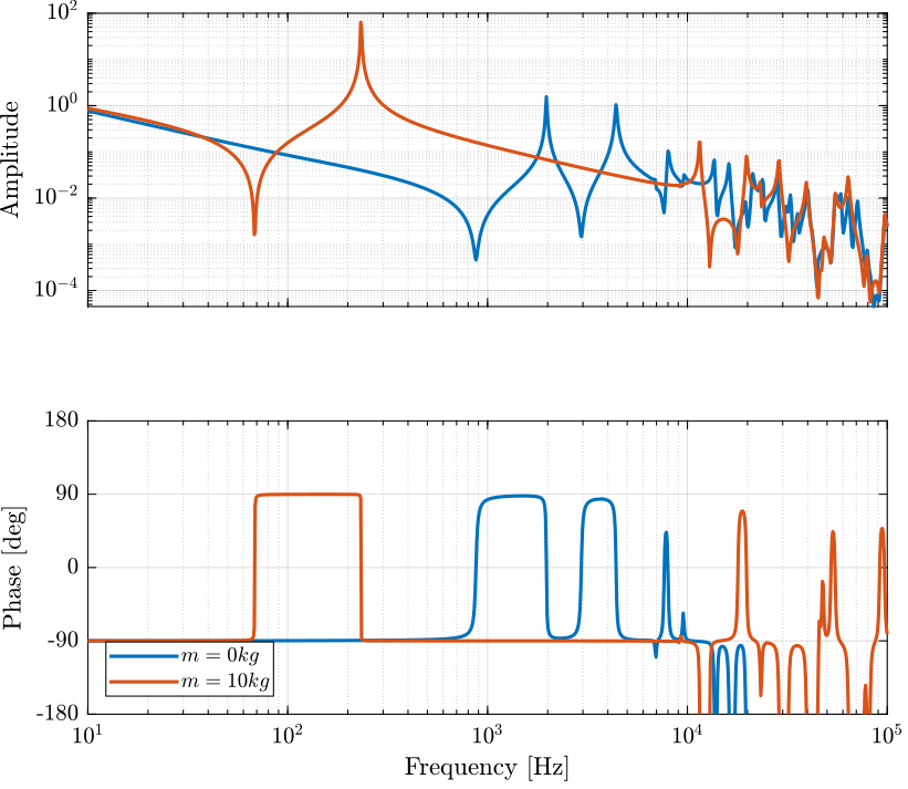
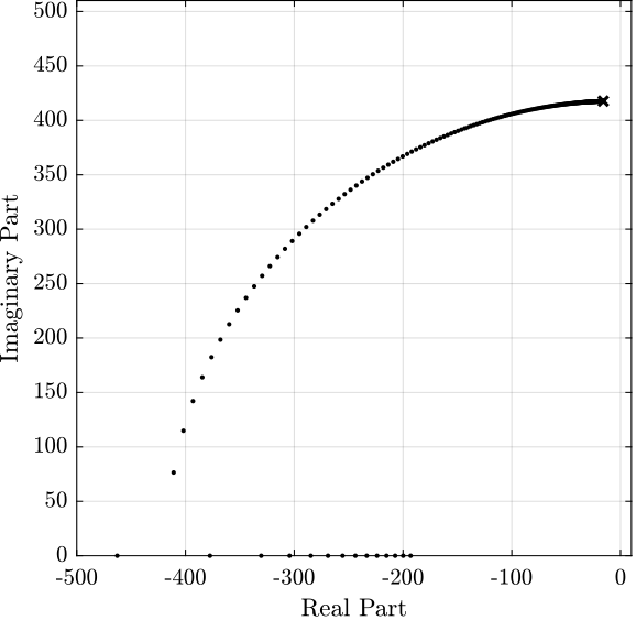
Figure 24: IFF Loop Gain
5.4 Closed Loop System
m = 10;
Kiff = -1e12/s;
%% Name of the Simulink File
mdl = 'piezo_amplified_IFF';

%% Input/Output definition
clear io; io_i = 1;
io(io_i) = linio([mdl, '/Dw'], 1, 'openinput');  io_i = io_i + 1;
io(io_i) = linio([mdl, '/F'],  1, 'openinput');  io_i = io_i + 1;
io(io_i) = linio([mdl, '/Fd'], 1, 'openinput');  io_i = io_i + 1;
io(io_i) = linio([mdl, '/d'],  1, 'openoutput'); io_i = io_i + 1;
io(io_i) = linio([mdl, '/G'],  1, 'output'); io_i = io_i + 1;

Giff = linearize(mdl, io);
Giff.InputName  = {'w', 'f', 'F'};
Giff.OutputName  = {'x1', 'Fs'};
Kiff = tf(0);
G = linearize(mdl, io);
G.InputName  = {'w', 'f', 'F'};
G.OutputName  = {'x1', 'Fs'};
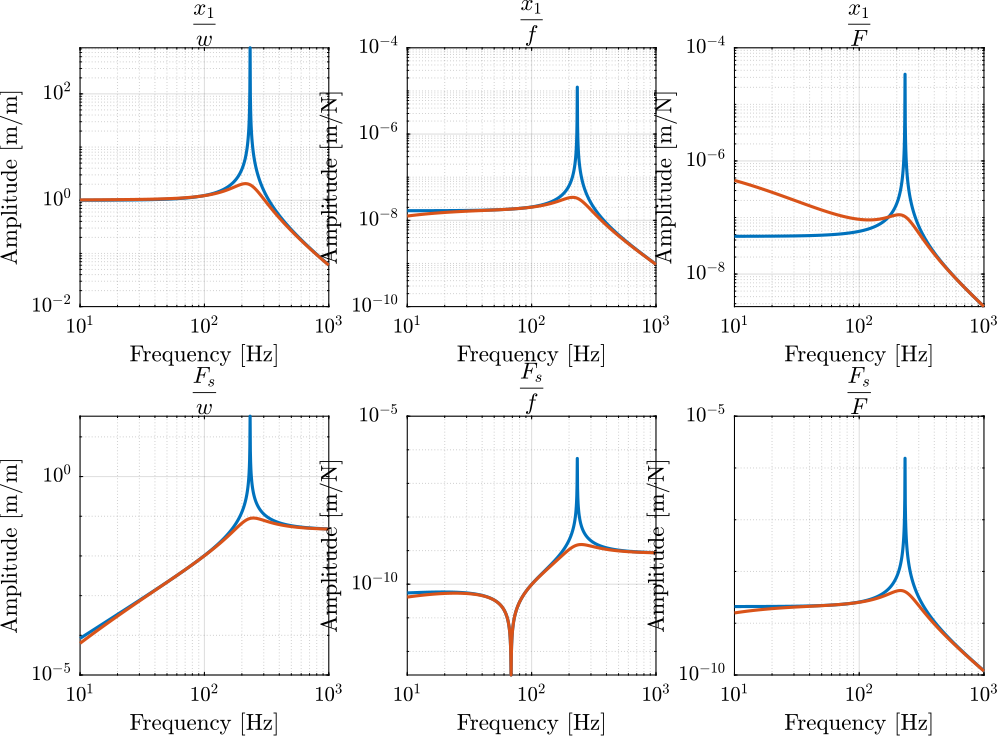
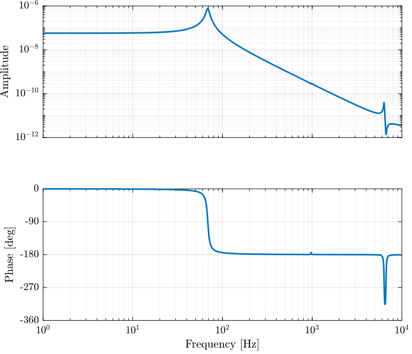
Figure 25: OL and CL transfer functions
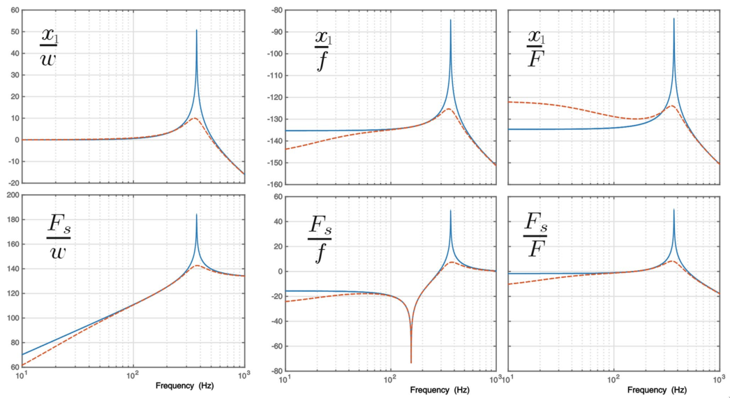
Figure 26: Results obtained in souleille18_concep_activ_mount_space_applic
6 Complete Strut with Encoder
6.1 Introduction

Figure 27: Interface points
Flexible joints have 0.25mm width.
6.2 Import Mass Matrix, Stiffness Matrix, and Interface Nodes Coordinates
We first extract the stiffness and mass matrices.
K = readmatrix('mat_K.CSV');
M = readmatrix('mat_M.CSV');
Then, we extract the coordinates of the interface nodes.
[int_xyz, int_i, n_xyz, n_i, nodes] = extractNodes('out_nodes_3D.txt');
save('./mat/strut_encoder.mat', 'int_xyz', 'int_i', 'n_xyz', 'n_i', 'nodes', 'M', 'K');
6.3 Output parameters
load('./mat/strut_encoder.mat', 'int_xyz', 'int_i', 'n_xyz', 'n_i', 'nodes', 'M', 'K');
| Total number of Nodes | 8 |
| Number of interface Nodes | 8 |
| Number of Modes | 6 |
| Size of M and K matrices | 54 |
| Node i | Node Number | x [m] | y [m] | z [m] |
|---|---|---|---|---|
| 1.0 | 504411.0 | 0.0 | 0.0 | 0.0405 |
| 2.0 | 504412.0 | 0.0 | 0.0 | -0.0405 |
| 3.0 | 504413.0 | -0.0325 | 0.0 | 0.0 |
| 4.0 | 504414.0 | -0.0125 | 0.0 | 0.0 |
| 5.0 | 504415.0 | -0.0075 | 0.0 | 0.0 |
| 6.0 | 504416.0 | 0.0325 | 0.0 | 0.0 |
| 7.0 | 504417.0 | 0.004 | 0.0145 | -0.00175 |
| 8.0 | 504418.0 | 0.004 | 0.0166 | -0.00175 |
| 2000000.0 | 1000000.0 | -3000000.0 | -400.0 | 300.0 | 200.0 | -30.0 | 2000.0 | -10000.0 | 0.3 |
| 1000000.0 | 4000000.0 | -8000000.0 | -900.0 | 400.0 | -50.0 | -6000.0 | 10000.0 | -20000.0 | 3 |
| -3000000.0 | -8000000.0 | 20000000.0 | 2000.0 | -900.0 | 200.0 | -10000.0 | 20000.0 | -300000.0 | 7 |
| -400.0 | -900.0 | 2000.0 | 5 | -0.1 | 0.05 | 1 | -3 | 6 | -0.0007 |
| 300.0 | 400.0 | -900.0 | -0.1 | 5 | 0.04 | -0.1 | 0.5 | -3 | 0.0001 |
| 200.0 | -50.0 | 200.0 | 0.05 | 0.04 | 300.0 | 4 | -0.01 | -1 | 3e-05 |
| -30.0 | -6000.0 | -10000.0 | 1 | -0.1 | 4 | 3000000.0 | -1000000.0 | -2000000.0 | -300.0 |
| 2000.0 | 10000.0 | 20000.0 | -3 | 0.5 | -0.01 | -1000000.0 | 6000000.0 | 7000000.0 | 1000.0 |
| -10000.0 | -20000.0 | -300000.0 | 6 | -3 | -1 | -2000000.0 | 7000000.0 | 20000000.0 | 2000.0 |
| 0.3 | 3 | 7 | -0.0007 | 0.0001 | 3e-05 | -300.0 | 1000.0 | 2000.0 | 5 |
| 0.04 | -0.005 | 0.007 | 2e-06 | 0.0001 | -5e-07 | -1e-05 | -9e-07 | 8e-05 | -5e-10 |
| -0.005 | 0.03 | 0.02 | -0.0001 | 1e-06 | -3e-07 | 3e-05 | -0.0001 | 8e-05 | -3e-08 |
| 0.007 | 0.02 | 0.08 | -6e-06 | -5e-06 | -7e-07 | 4e-05 | -0.0001 | 0.0005 | -3e-08 |
| 2e-06 | -0.0001 | -6e-06 | 2e-06 | -4e-10 | 2e-11 | -8e-09 | 3e-08 | -2e-08 | 6e-12 |
| 0.0001 | 1e-06 | -5e-06 | -4e-10 | 3e-06 | 2e-10 | -3e-09 | 3e-09 | -7e-09 | 6e-13 |
| -5e-07 | -3e-07 | -7e-07 | 2e-11 | 2e-10 | 5e-07 | -2e-08 | 5e-09 | -5e-09 | 1e-12 |
| -1e-05 | 3e-05 | 4e-05 | -8e-09 | -3e-09 | -2e-08 | 0.04 | 0.004 | 0.003 | 1e-06 |
| -9e-07 | -0.0001 | -0.0001 | 3e-08 | 3e-09 | 5e-09 | 0.004 | 0.02 | -0.02 | 0.0001 |
| 8e-05 | 8e-05 | 0.0005 | -2e-08 | -7e-09 | -5e-09 | 0.003 | -0.02 | 0.08 | -5e-06 |
| -5e-10 | -3e-08 | -3e-08 | 6e-12 | 6e-13 | 1e-12 | 1e-06 | 0.0001 | -5e-06 | 2e-06 |
Using K, M and int_xyz, we can use the Reduced Order Flexible Solid simscape block.
6.4 Piezoelectric parameters
Parameters for the APA300ML:
d33 = 3e-10; % Strain constant [m/V]
n = 80; % Number of layers per stack
eT = 1.6e-8; % Permittivity under constant stress [F/m]
sD = 2e-11; % Elastic compliance under constant electric displacement [m2/N]
ka = 235e6; % Stack stiffness [N/m]
C = 5e-6; % Stack capactiance [F]
na = 2; % Number of stacks used as actuator
ns = 1; % Number of stacks used as force sensor
6.5 Identification of the Dynamics
The dynamics is identified from the applied force to the measured relative displacement. The same dynamics is identified for a payload mass of 10Kg.
m = 10;