Robust Control - \(\mathcal{H}_\infty\) Synthesis
Table of Contents
1 Introduction to the Control Methodology - Model Based Control
1.1 Control Methodology
The typical methodology when applying Model Based Control to a plant is schematically shown in Figure 1. It consists of three steps:
- Identification or modeling: \(\Longrightarrow\) mathematical model
- Translate the specifications into mathematical criteria:
- Specifications: Response Time, Noise Rejection, Maximum input amplitude, Robustness, …
- Mathematical Criteria: Cost Function, Shape of TF
- Synthesis: research of \(K\) that satisfies the specifications for the model of the system
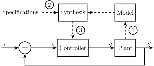
Figure 1: Typical Methodoly for Model Based Control
In this document, we will mainly focus on steps 2 and 3.
1.2 Some Background: From Classical Control to Robust Control
| Classical Control | Modern Control | Robust Control | |
|---|---|---|---|
| Date | 1930- | 1960- | 1980- |
| Tools | Transfer Functions | State Space formulation | Systems and Signals Norms (\(\mathcal{H}_\infty\), \(\mathcal{H}_2\) Norms) |
| Nyquist Plots | Riccati Equations | Closed Loop Transfer Functions | |
| Bode Plots | Open/Closed Loop Shaping | ||
| Phase and Gain margins | Weighting Functions | ||
| Disk margin | |||
| Control Architectures | Proportional, Integral, Derivative | Full State Feedback | General Control Configuration |
| Leads, Lags | LQR, LQG | ||
| Kalman Filters | |||
| Advantages | Study Stability | Automatic Synthesis | Automatic Synthesis |
| Simple | MIMO | MIMO | |
| Natural | Optimization Problem | Optimization Problem | |
| Guaranteed Robustness | |||
| Easy specification of performances | |||
| Disadvantages | Manual Method | No Guaranteed Robustness | Required knowledge of specific tools |
| Only SISO | Difficult Rejection of Perturbations | Need a reasonably good model of the system |
1.3 Example System
Let’s consider the model shown in Figure 2. It could represent a suspension system with a payload to position or isolate using an force actuator and an inertial sensor. The notations used are listed in Table 2.
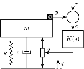
Figure 2: Test System consisting of a payload with a mass \(m\) on top of an active system with a stiffness \(k\), damping \(c\) and an actuator. A feedback controller \(K(s)\) is added to position / isolate the payload.
| Notation | Description | Value | Unit |
|---|---|---|---|
| \(m\) | Payload’s mass to position / isolate | \(10\) | [kg] |
| \(k\) | Stiffness of the suspension system | \(10^6\) | [N/m] |
| \(c\) | Damping coefficient of the suspension system | \(400\) | [N/(m/s)] |
| \(y\) | Payload absolute displacement (measured by an inertial sensor) | [m] | |
| \(d\) | Ground displacement, it acts as a disturbance | [m] | |
| \(u\) | Actuator force | [N] | |
| \(r\) | Wanted position of the mass (the reference) | [m] | |
| \(\epsilon = r - y\) | Position error | [m] | |
| \(K\) | Feedback controller | to be designed | [N/m] |
Derive the following open-loop transfer functions:
\begin{align} G(s) &= \frac{y}{u} \\ G_d(s) &= \frac{y}{d} \end{align}Hint
You can follow this generic procedure:
- List all applied forces ot the mass: Actuator force, Stiffness force (Hooke’s law), …
- Apply the Newton’s Second Law on the payload \[ m \ddot{y} = \Sigma F \]
- Transform the differential equations into the Laplace domain: \[ \frac{d\ \cdot}{dt} \Leftrightarrow \cdot \times s \]
- Write \(y(s)\) as a function of \(u(s)\) and \(w(s)\)
Results
\begin{align} G(s) &= \frac{1}{m s^2 + cs + k} \\ G_d(s) &= \frac{cs + k}{m s^2 + cs + k} \end{align}Having obtained \(G(s)\) and \(G_d(s)\), we can transform the system shown in Figure 2 into a classical feedback form as shown in Figure 6.
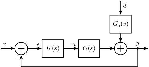
Figure 3: Block diagram corresponding to the example system
Let’s define the system parameters on Matlab.
1: k = 1e6; % Stiffness [N/m]
2: c = 4e2; % Damping [N/(m/s)]
3: m = 10; % Mass [kg]
And now the system dynamics \(G(s)\) and \(G_d(s)\) (their bode plots are shown in Figures 4 and 5).
4: G = 1/(m*s^2 + c*s + k); % Plant
5: Gd = (c*s + k)/(m*s^2 + c*s + k); % Disturbance

Figure 4: Bode plot of the plant \(G(s)\)
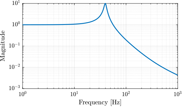
Figure 5: Magnitude of the disturbance transfer function \(G_d(s)\)
2 Classical Open Loop Shaping
2.1 Introduction to Open Loop Shaping
The Loop Gain \(L(s)\) usually refers to as the product of the controller and the plant (Figure 6):
\begin{equation} L(s) = G(s) \cdot K(s) \label{eq:loop_gain} \end{equation}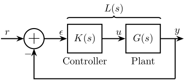
Figure 6: Classical Feedback Architecture
Open Loop Shaping refers to a control design technique where the controller \(K(s)\) is designed such that the Open Loop Gain \(L(s)\) has desirable shape.
This synthesis method is widely used as many characteristics of the closed-loop system depend on the shape of the open loop gain \(L(s)\):
- Performance: \(L\) large
- Good disturbance rejection: \(L\) large
- Limitation of measurement noise on plant output: \(L\) small
- Small magnitude of input signal: \(K\) and \(L\) small
- Nominal stability: \(L\) small (RHP zeros and time delays)
- Robust stability: \(L\) small (neglected dynamics)
The Open Loop shape is usually done manually has the loop gain \(L(s)\) depends linearly on \(K(s)\) \eqref{eq:loop_gain}.
\(K(s)\) then consists of a combination of leads, lags, notches, etc. such that \(L(s)\) has the wanted shape.
2.2 Example of Open Loop Shaping
Let’s take our example system and try to apply the Open-Loop shaping strategy to design a controller that fulfils the following specifications:
- Performance: Bandwidth of approximately 10Hz
- Noise Attenuation: Roll-off of -40dB/decade past 30Hz
- Robustness: Gain margin > 3dB and Phase margin > 30 deg
Using SISOTOOL, design a controller that fulfill the specifications.
sisotool(G)
In order to have the wanted Roll-off, two integrators are used, a lead is also added to have sufficient phase margin.
The obtained controller is shown below, and the bode plot of the Loop Gain is shown in Figure 7.
K = 14e8 * ... % Gain
    1/(s^2) * ... % Double Integrator
    1/(1 + s/2/pi/40) * ... % Low Pass Filter
    (1 + s/(2*pi*10/sqrt(8)))/(1 + s/(2*pi*10*sqrt(8))); % Lead
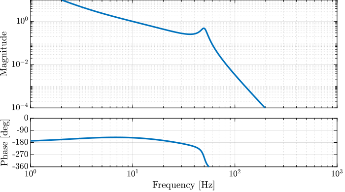
Figure 7: Bode Plot of the obtained Loop Gain \(L(s) = G(s) K(s)\)
And we can verify that we have the wanted stability margins:
[Gm, Pm, ~, Wc] = margin(G*K)
| Manual Method | |
|---|---|
| Gain Margin \(> 3\) [dB] | 3.1 |
| Phase Margin \(> 30\) [deg] | 35.4 |
| Crossover \(\approx 10\) [Hz] | 10.1 |
2.3 \(\mathcal{H}_\infty\) Loop Shaping Synthesis
The Open Loop Shaping synthesis can be performed using the \(\mathcal{H}_\infty\) Synthesis.
Even though we will not go into details, we will provide one example.
Using Matlab, the \(\mathcal{H}_\infty\) synthesis of a controller based on the wanted open loop shape can be performed using the loopsyn command:
K = loopsyn(G, Gd);
where:
Gis the (LTI) plantGdis the wanted loop shapeKis the synthesize controller
Matlab documentation of loopsyn (link).
2.4 Example of the \(\mathcal{H}_\infty\) Loop Shaping Synthesis
Let’s reuse the previous plant.
Translate the specification into the wanted shape of the open loop gain.
- Performance: Bandwidth of approximately 10Hz: \(|L_w(j2 \pi 10)| = 1\)
- Noise Attenuation: Roll-off of -40dB/decade past 30Hz
- Robustness: Gain margin > 3dB and Phase margin > 30 deg
Lw = 2.3e3 * ...
     1/(s^2) * ... % Double Integrator
     (1 + s/(2*pi*10/sqrt(3)))/(1 + s/(2*pi*10*sqrt(3))); % Lead
The \(\mathcal{H}_\infty\) optimal open loop shaping is performed using the loopsyn command:
[K, ~, GAM] = loopsyn(G, Lw);
The Bode plot of the obtained controller is shown in Figure 8.
It is always important to analyze the controller after the synthesis is performed.
In the end, a synthesize controller is just a combination of low pass filters, high pass filters, notches, leads, etc.
Let’s briefly analyze this controller:
- two integrators are used at low frequency to have the wanted low frequency high gain
- a lead is added centered with the crossover frequency to increase the phase margin
- a notch is added at the resonance of the plant to increase the gain margin (this is very typical of \(\mathcal{H}_\infty\) controllers, and can be an issue, more info on that latter)
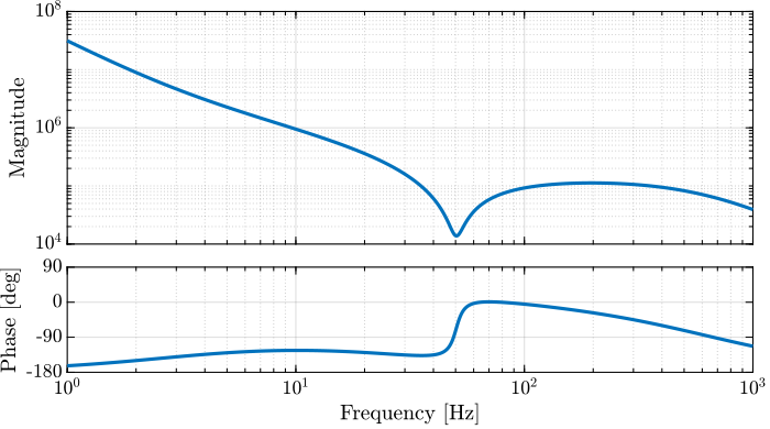
Figure 8: Obtained controller \(K\) using the open-loop \(\mathcal{H}_\infty\) shaping
The obtained Loop Gain is shown in Figure 9.
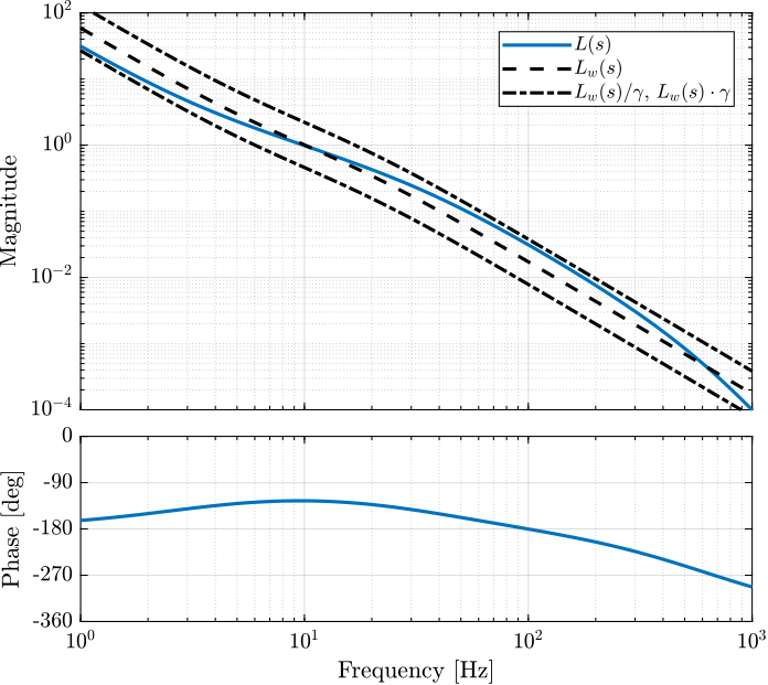
Figure 9: Obtained Open Loop Gain \(L(s) = G(s) K(s)\) and comparison with the wanted Loop gain \(L_w\)
Let’s now compare the obtained stability margins of the \(\mathcal{H}_\infty\) controller and of the manually developed controller in Table 3.
| Specifications | Manual Method | \(\mathcal{H}_\infty\) Method |
|---|---|---|
| Gain Margin \(> 3\) [dB] | 3.1 | 31.7 |
| Phase Margin \(> 30\) [deg] | 35.4 | 54.7 |
| Crossover \(\approx 10\) [Hz] | 10.1 | 9.9 |
3 First Step in the \(\mathcal{H}_\infty\) world
3.1 The \(\mathcal{H}_\infty\) Norm
The \(\mathcal{H}_\infty\) norm is defined as the peak of the maximum singular value of the frequency response
\begin{equation} \|G(s)\|_\infty = \max_\omega \bar{\sigma}\big( G(j\omega) \big) \end{equation}For a SISO system \(G(s)\), it is simply the peak value of \(|G(j\omega)|\) as a function of frequency:
\begin{equation} \|G(s)\|_\infty = \max_{\omega} |G(j\omega)| \label{eq:hinf_norm_siso} \end{equation}
And compute its \(\mathcal{H}_\infty\) norm using the hinfnorm function:
hinfnorm(G)
7.9216e-06
The magnitude \(|G(j\omega)|\) of the plant \(G(s)\) as a function of frequency is shown in Figure 10. The maximum value of the magnitude over all frequencies does correspond to the \(\mathcal{H}_\infty\) norm of \(G(s)\) as Equation \eqref{eq:hinf_norm_siso} implies.

Figure 10: Example of the \(\mathcal{H}_\infty\) norm of a SISO system
3.2 \(\mathcal{H}_\infty\) Synthesis
Optimization problem: \(\mathcal{H}_\infty\) synthesis is a method that uses an algorithm (LMI optimization, Riccati equation) to find a controller of the same order as the system so that the \(\mathcal{H}_\infty\) norms of defined transfer functions are minimized.
Engineer work:
- Write the problem as standard \(\mathcal{H}_\infty\) problem
- Translate the specifications as \(\mathcal{H}_\infty\) norms
- Make the synthesis and analyze the obtain controller
- Reduce the order of the controller for implementation
Many ways to use the \(\mathcal{H}_\infty\) Synthesis:
- Traditional \(\mathcal{H}_\infty\) Synthesis
- Mixed Sensitivity Loop Shaping
- Fixed-Structure \(\mathcal{H}_\infty\) Synthesis
- Signal Based \(\mathcal{H}_\infty\) Synthesis
3.3 The Generalized Plant
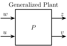
| Notation | Meaning |
|---|---|
| \(P\) | Generalized plant model |
| \(w\) | Exogenous inputs: commands, disturbances, noise |
| \(z\) | Exogenous outputs: signals to be minimized |
| \(v\) | Controller inputs: measurements |
| \(u\) | Control signals |
3.4 From a Classical Feedback Architecture to a Generalized Plant

Figure 12: Classical Feedback Architecture
| Notation | Meaning |
|---|---|
| \(G\) | Plant model |
| \(K\) | Controller |
| \(r\) | Reference inputs |
| \(y\) | Plant outputs |
| \(u\) | Control signals |
| \(d\) | Input Disturbance |
| \(\epsilon\) | Tracking Error |
The procedure is:
- define signals of the generalized plant
- Remove \(K\) and rearrange the inputs and outputs
Let’s find the Generalized plant of corresponding to the tracking control architecture shown in Figure 13
![]()
Figure 13: Classical Feedback Control Architecture (Tracking)
First, define the signals of the generalized plant:
- Exogenous inputs: \(w = r\)
- Signals to be minimized: \(z_1 = \epsilon\), \(z_2 = u\)
- Control signals: \(v = y\)
- Control inputs: \(u\)
Then, Remove \(K\) and rearrange the inputs and outputs. We obtain the generalized plant shown in Figure 14.
![]()
Figure 14: Generalized plant of the Classical Feedback Control Architecture (Tracking)
Using Matlab, the generalized plant can be defined as follows:
P = [1 -G;
     0  1;
     1 -G]
3.5 The General Synthesis Problem Formulation
The \(\mathcal{H}_\infty\) Synthesis objective is to find all stabilizing controllers \(K\) which minimize
\begin{equation} \| F_l(P, K) \|_\infty = \max_{\omega} \overline{\sigma} \big( F_l(P, K)(j\omega) \big) \end{equation}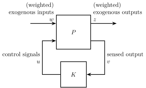
Figure 15: General Control Configuration
4 Modern Interpretation of the Control Specifications
4.1 Introduction
- Reference tracking Overshoot, Static error, Setling time
- \(S(s) = T_{r \rightarrow \epsilon}\)
- Disturbances rejection
- \(G(s) S(s) = T_{d \rightarrow \epsilon}\)
- Measurement noise filtering
- \(T(s) = T_{n \rightarrow \epsilon}\)
- Small command amplitude
- \(K(s) S(s) = T_{r \rightarrow u}\)
- Stability
- \(S(s)\), \(T(s)\), \(K(s)S(s)\), \(G(s)S(s)\)
- Robustness to plant uncertainty (stability margins)
- Controller implementation
**
5 Resources