Robust Control - \(\mathcal{H}_\infty\) Synthesis
Table of Contents
- 1. Introduction to the Control Methodology - Model Based Control
- 2. Some Background: From Classical Control to Robust Control
- 3. The \(\mathcal{H}_\infty\) Norm
- 4. \(\mathcal{H}_\infty\) Synthesis
- 5. The Generalized Plant
- 6. Problem Formulation
- 7. Classical feedback control and closed loop transfer functions
- 8. From a Classical Feedback Architecture to a Generalized Plant
- 9. Modern Interpretation of the Control Specifications
- 10. Resources
1 Introduction to the Control Methodology - Model Based Control
The typical methodology when applying Model Based Control to a plant is schematically shown in Figure 1. It consists of three steps:
- Identification or modeling: \(\Longrightarrow\) mathematical model
- Translate the specifications into mathematical criteria:
- Specifications: Response Time, Noise Rejection, Maximum input amplitude, Robustness, …
- Mathematical Criteria: Cost Function, Shape of TF
- Synthesis: research of \(K\) that satisfies the specifications for the model of the system
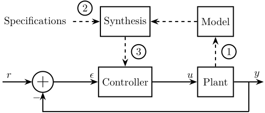
Figure 1: Typical Methodoly for Model Based Control
In this document, we will mainly focus on steps 2 and 3.
2 Some Background: From Classical Control to Robust Control
Classical Control (1930)
- Tools:
- TF (input-output)
- Nyquist, Bode, Black, \ldots
- P-PI-PID, Phase lead-lag, \ldots
- Advantages:
- Stability
- Performances
- Robustness
- Disadvantages:
- Manual Method
- Only SISO
Modern Control (1960)
- Tools:
- State Space
- Optimal Command
- LQR, LQG
- Advantages:
- Automatic Synthesis
- MIMO
- Optimisation problem
- Disadvantages:
- Robustness
- Rejection of Perturbations
Robust Control (1980)
- Tools:
- Disk Margin
- Systems and Signals norms (\(\mathcal{H}_\infty\) and \(\mathcal{H}_2\) norms)
- Closed Loop Transfer Functions
- Loop Shaping
- Advantages:
- Stability
- Performances
- Robustness
- Automatic Synthesis
- MIMO
- Optimization Problem
- Disadvantages:
- Requires the knowledge of specific tools
- Need a reasonably good model of the system
3 The \(\mathcal{H}_\infty\) Norm
The \(\mathcal{H}_\infty\) norm is defined as the peak of the maximum singular value of the frequency response
\begin{equation} \|G(s)\|_\infty = \max_\omega \bar{\sigma}\big( G(j\omega) \big) \end{equation}For a SISO system \(G(s)\), it is simply the peak value of \(|G(j\omega)|\) as a function of frequency:
\begin{equation} \|G(s)\|_\infty = \max_{\omega} |G(j\omega)| \label{eq:hinf_norm_siso} \end{equation}Let’s define a plant dynamics:
w0 = 2*pi; k = 1e6; xi = 0.04;

G = 1/k/(s^2/w0^2 + 2*xi*s/w0 + 1);
And compute its \(\mathcal{H}_\infty\) norm using the hinfnorm function:
hinfnorm(G)
1.0013e-05
The magnitude \(|G(j\omega)|\) of the plant \(G(s)\) as a function of frequency is shown in Figure 2. The maximum value of the magnitude over all frequencies does correspond to the \(\mathcal{H}_\infty\) norm of \(G(s)\) as Equation \eqref{eq:hinf_norm_siso} implies.
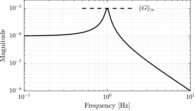
Figure 2: Example of the \(\mathcal{H}_\infty\) norm of a SISO system
4 \(\mathcal{H}_\infty\) Synthesis
Optimization problem: \(\hinf\) synthesis is a method that uses an algorithm (LMI optimization, Riccati equation) to find a controller of the same order as the system so that the \(\hinf\) norms of defined transfer functions are minimized.
Engineer work:
- Write the problem as standard \(\hinf\) problem
- Translate the specifications as \(\hinf\) norms
- Make the synthesis and analyze the obtain controller
- Reduce the order of the controller for implementation
Many ways to use the \(\hinf\) Synthesis:
- Traditional \(\hinf\) Synthesis
- Mixed Sensitivity Loop Shaping
- Fixed-Structure \(\hinf\) Synthesis
- Signal Based \(\hinf\) Synthesis
5 The Generalized Plant
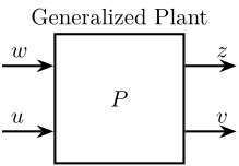
| Notation | Meaning |
|---|---|
| \(P\) | Generalized plant model |
| \(w\) | Exogenous inputs: commands, disturbances, noise |
| \(z\) | Exogenous outputs: signals to be minimized |
| \(v\) | Controller inputs: measurements |
| \(u\) | Control signals |
6 Problem Formulation
The \(\mathcal{H}_\infty\) Synthesis objective is to find all stabilizing controllers \(K\) which minimize
\begin{equation} \| F_l(P, K) \|_\infty = \max_{\omega} \overline{\sigma} \big( F_l(P, K)(j\omega) \big) \end{equation}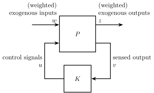
Figure 4: General Control Configuration
7 Classical feedback control and closed loop transfer functions
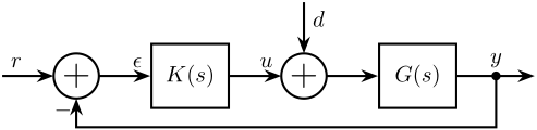
Figure 5: Classical Feedback Architecture
| Notation | Meaning |
|---|---|
| \(G\) | Plant model |
| \(K\) | Controller |
| \(r\) | Reference inputs |
| \(y\) | Plant outputs |
| \(u\) | Control signals |
| \(d\) | Input Disturbance |
| \(\epsilon\) | Tracking Error |
8 From a Classical Feedback Architecture to a Generalized Plant
The procedure is:
- define signals of the generalized plant
- Remove \(K\) and rearrange the inputs and outputs
Let’s find the Generalized plant of corresponding to the tracking control architecture shown in Figure 6
![]()
Figure 6: Classical Feedback Control Architecture (Tracking)
First, define the signals of the generalized plant:
- Exogenous inputs: \(w = r\)
- Signals to be minimized: \(z_1 = \epsilon\), \(z_2 = u\)
- Control signals: \(v = y\)
- Control inputs: \(u\)
Then, Remove \(K\) and rearrange the inputs and outputs. We obtain the generalized plant shown in Figure 7.
![]()
Figure 7: Generalized plant of the Classical Feedback Control Architecture (Tracking)
Using Matlab, the generalized plant can be defined as follows:
P = [1 -G;
     0  1;
     1 -G]
9 Modern Interpretation of the Control Specifications
9.1 Introduction
- Reference tracking Overshoot, Static error, Setling time
- \(S(s) = T_{r \rightarrow \epsilon}\)
- Disturbances rejection
- \(G(s) S(s) = T_{d \rightarrow \epsilon}\)
- Measurement noise filtering
- \(T(s) = T_{n \rightarrow \epsilon}\)
- Small command amplitude
- \(K(s) S(s) = T_{r \rightarrow u}\)
- Stability
- \(S(s)\), \(T(s)\), \(K(s)S(s)\), \(G(s)S(s)\)
- Robustness to plant uncertainty (stability margins)
- Controller implementation
**
10 Resources