Encoder - Test Bench

1. Experimental Setup
2. Huddle Test
3. Comparison Interferometer / Encoder
4. Identification
- 4.1. Load Data
- 4.2. Identification

1 Experimental Setup

The experimental Setup is schematically represented in Figure 1.

The mass can be vertically moved using the amplified piezoelectric actuator. The displacement of the mass (relative to the mechanical frame) is measured both by the interferometer and by the encoder.

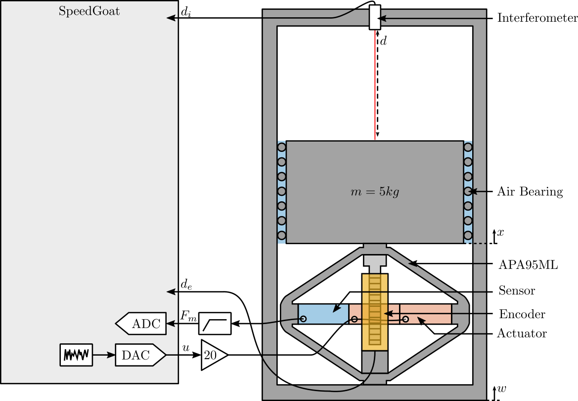
Figure 1: Schematic of the Experiment

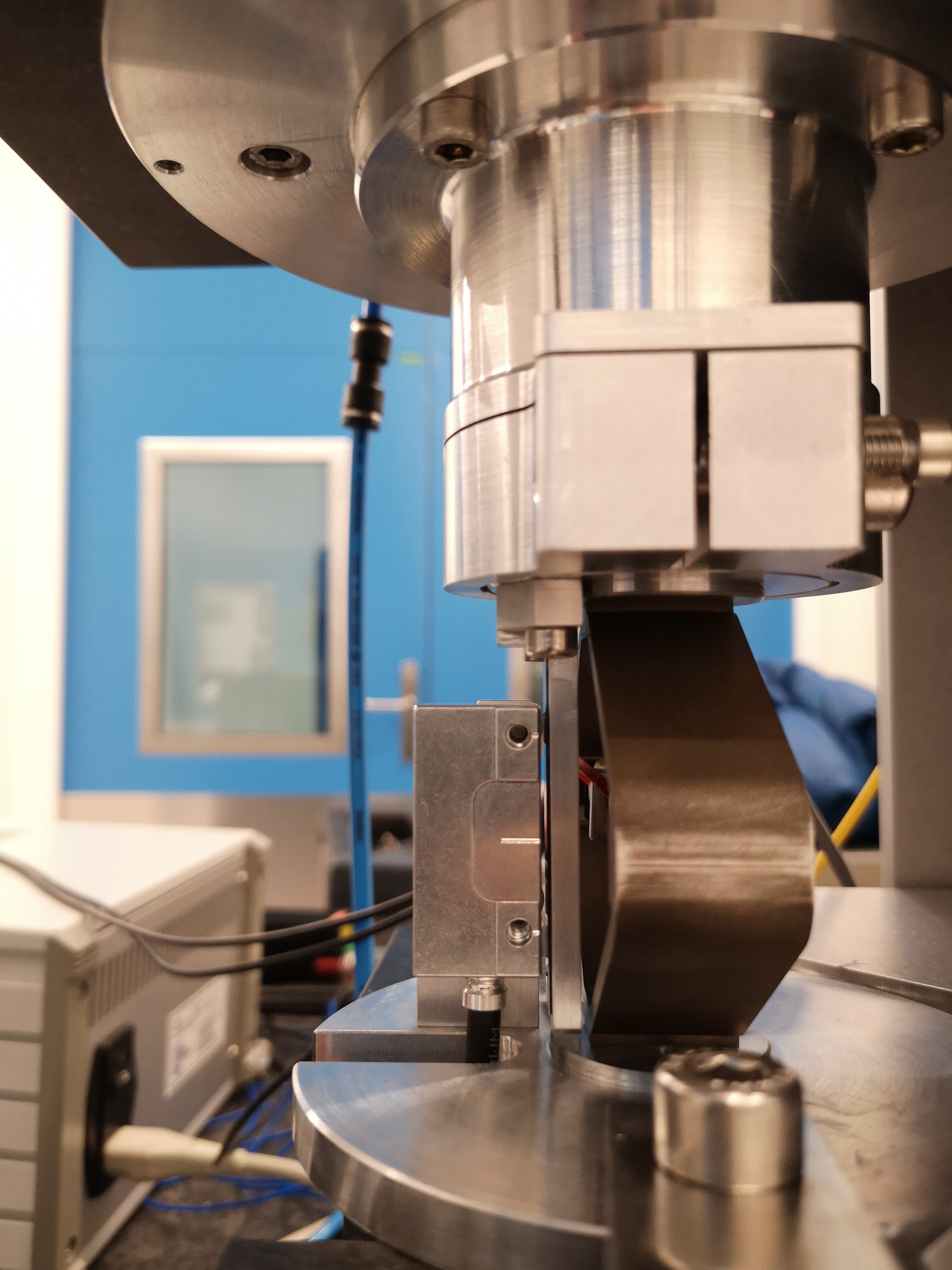
Figure 2: Side View of the encoder

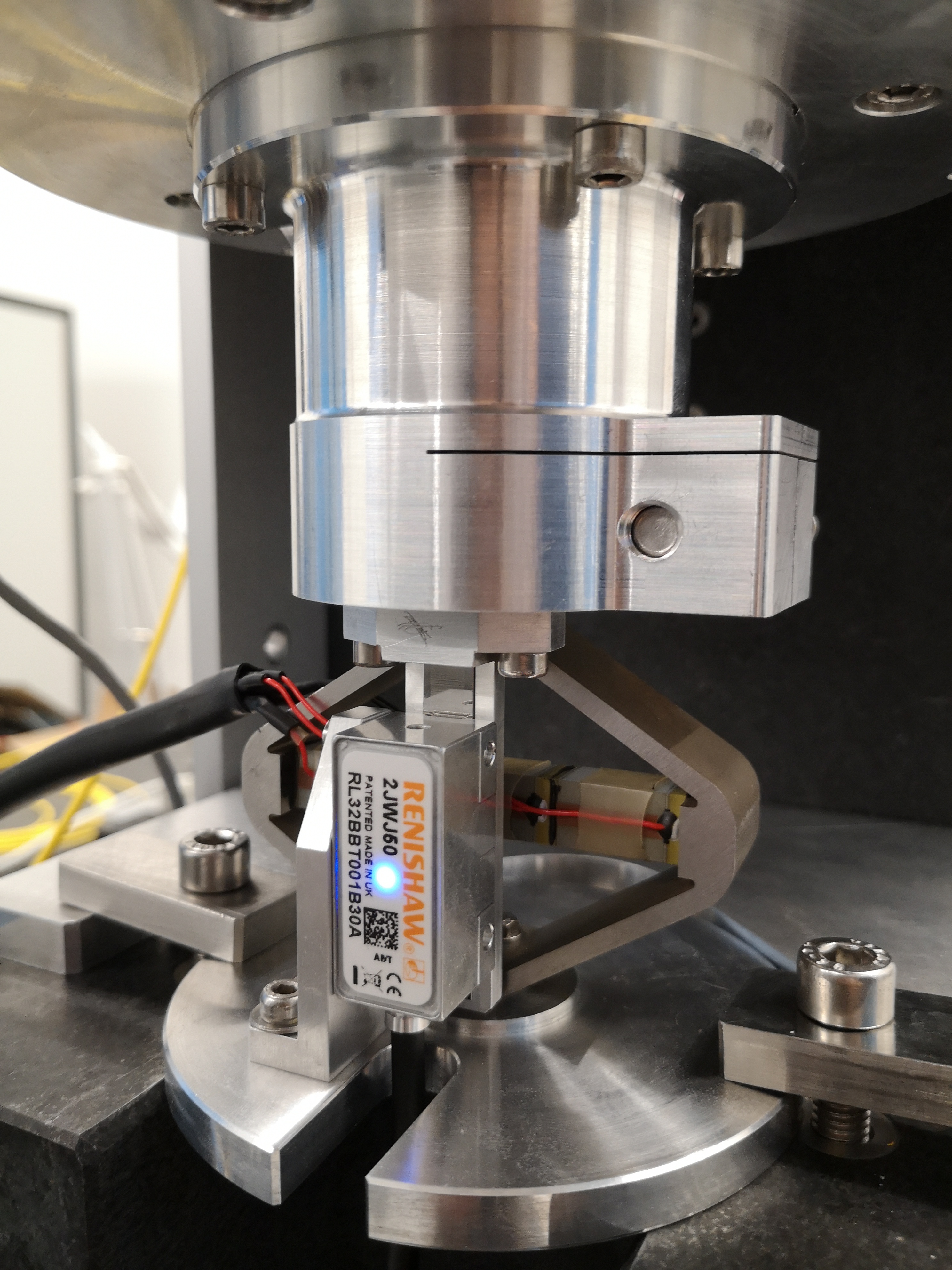
Figure 3: Front View of the encoder

2 Huddle Test

The goal in this section is the estimate the noise of both the encoder and the intereferometer.

Nothing is then to the actuator such that the relative motion between the mass and the frame is as small as possible. Ideally, a mechanical part would clamp the two together, we here suppose that the APA is still enough to clamp the two together.

2.1 Load Data

load('mat/int_enc_huddle_test.mat', 'interferometer', 'encoder', 't');

interferometer = detrend(interferometer, 0);
encoder = detrend(encoder, 0);

2.2 Time Domain Results

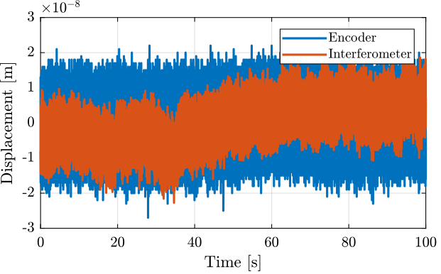
Figure 4: Huddle test - Time domain signals

G_lpf = 1/(1 + s/2/pi/10);

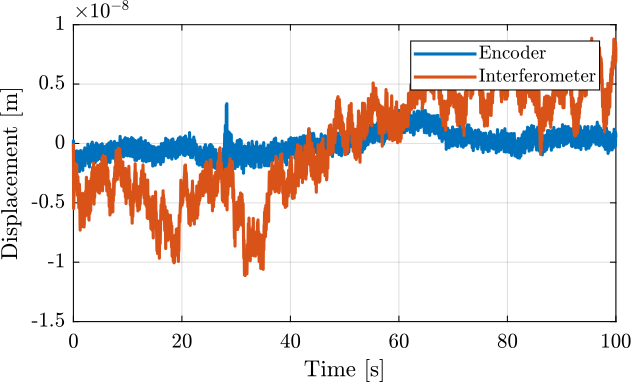
Figure 5: Huddle test - Time domain signals filtered with a LPF at 10Hz

2.3 Frequency Domain Noise

Ts = 1e-4;
win = hann(ceil(10/Ts));

[p_i, f] = pwelch(interferometer, win, [], [], 1/Ts);
[p_e, ~] = pwelch(encoder,        win, [], [], 1/Ts);

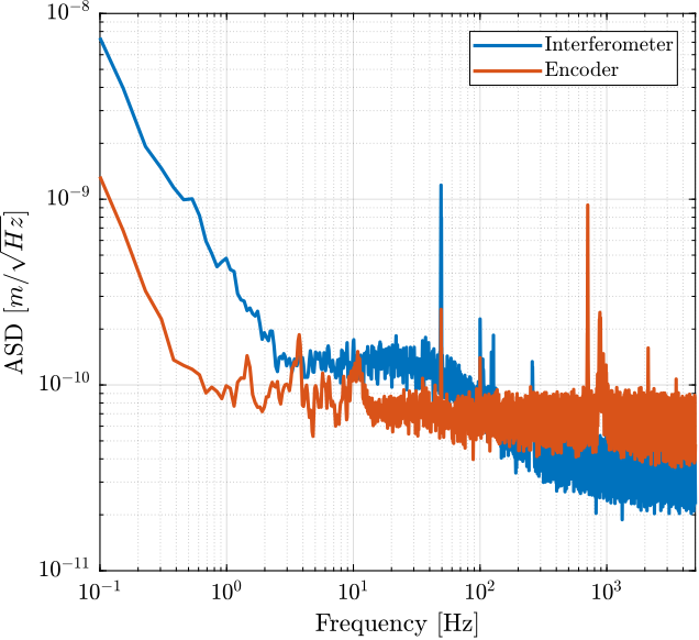
Figure 6: Amplitude Spectral Density of the signals during the Huddle test

3 Comparison Interferometer / Encoder

The goal here is to make sure that the interferometer and encoder measurements are coherent. We may see non-linearity in the interferometric measurement.

3.1 Load Data

load('mat/int_enc_comp.mat', 'interferometer', 'encoder', 'u', 't');

interferometer = detrend(interferometer, 0);
encoder = detrend(encoder, 0);
u = detrend(u, 0);

3.2 Time Domain Results

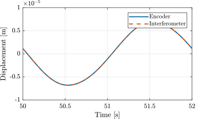
Figure 7: One cycle measurement

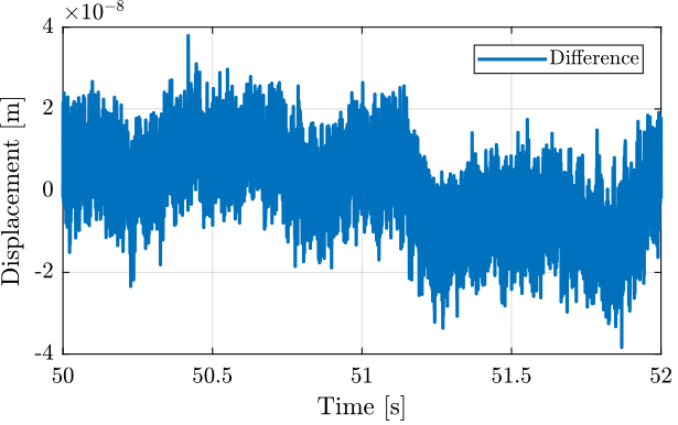
Figure 8: Difference between the Encoder and the interferometer during one cycle

3.3 Difference between Encoder and Interferometer as a function of time

Ts = 1e-4;
d_i_mean = reshape(interferometer, [2/Ts floor(Ts/2*length(interferometer))]);
d_e_mean = reshape(encoder,        [2/Ts floor(Ts/2*length(encoder))]);

w0 = 2*pi*5; % [rad/s]
xi = 0.7;

G_lpf = 1/(1 + 2*xi/w0*s + s^2/w0^2);

d_err_mean = reshape(lsim(G_lpf, encoder - interferometer, t), [2/Ts floor(Ts/2*length(encoder))]);
d_err_mean = d_err_mean - mean(d_err_mean);

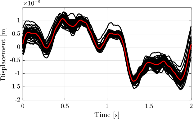
Figure 9: Difference between the two measurement in the time domain, averaged for all the cycles

3.4 Difference between Encoder and Interferometer as a function of position

Compute the mean of the interferometer measurement corresponding to each of the encoder measurement.

[e_sorted, ~, e_ind] = unique(encoder);

i_mean = zeros(length(e_sorted), 1);
for i = 1:length(e_sorted)
  i_mean(i) = mean(interferometer(e_ind == i));
end

i_mean_error = (i_mean - e_sorted);

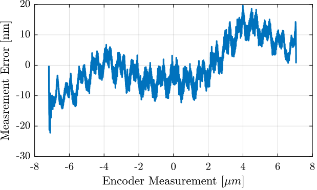
Figure 10: Difference between the two measurement as a function of the measured position by the encoder, averaged for all the cycles

The period of the non-linearity seems to be \(1.53 \mu m\) which corresponds to the wavelength of the Laser.

win_length = 1530; % length of the windows (corresponds to 1.53 um)
num_avg = floor(length(e_sorted)/win_length); % number of averaging

i_init = ceil((length(e_sorted) - win_length*num_avg)/2); % does not start at the extremity

e_sorted_mean_over_period = mean(reshape(i_mean_error(i_init:i_init+win_length*num_avg-1), [win_length num_avg]), 2);

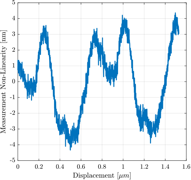
Figure 11: Non-Linearity of the Interferometer over the period of the wavelength

4 Identification

4.1 Load Data

load('mat/int_enc_id_noise_bis.mat', 'interferometer', 'encoder', 'u', 't');

interferometer = detrend(interferometer, 0);
encoder = detrend(encoder, 0);
u = detrend(u, 0);

4.2 Identification

Ts = 1e-4; % Sampling Time [s]
win = hann(ceil(10/Ts));

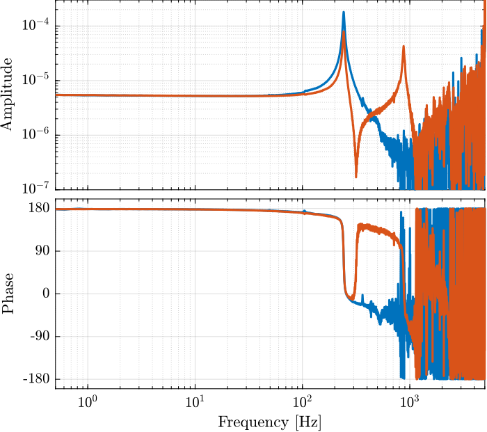
[tf_i_est, f] = tfestimate(u, interferometer, win, [], [], 1/Ts);
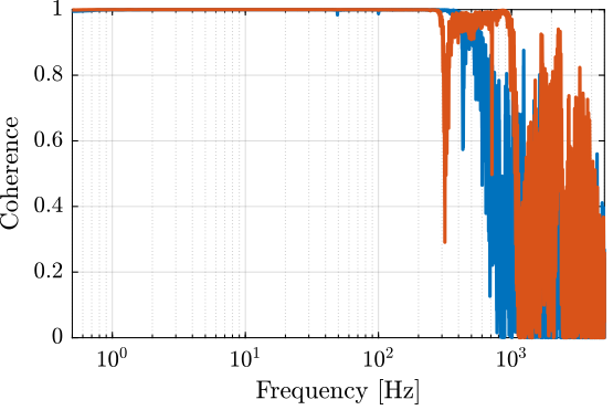
[co_i_est, ~] = mscohere(u, interferometer, win, [], [], 1/Ts);

[tf_e_est, ~] = tfestimate(u, encoder, win, [], [], 1/Ts);
[co_e_est, ~] = mscohere(u, encoder, win, [], [], 1/Ts);