Encoder - Test Bench
Table of Contents
1 Experimental Setup
The experimental Setup is schematically represented in Figure 1.
The mass can be vertically moved using the amplified piezoelectric actuator. The displacement of the mass (relative to the mechanical frame) is measured both by the interferometer and by the encoder.
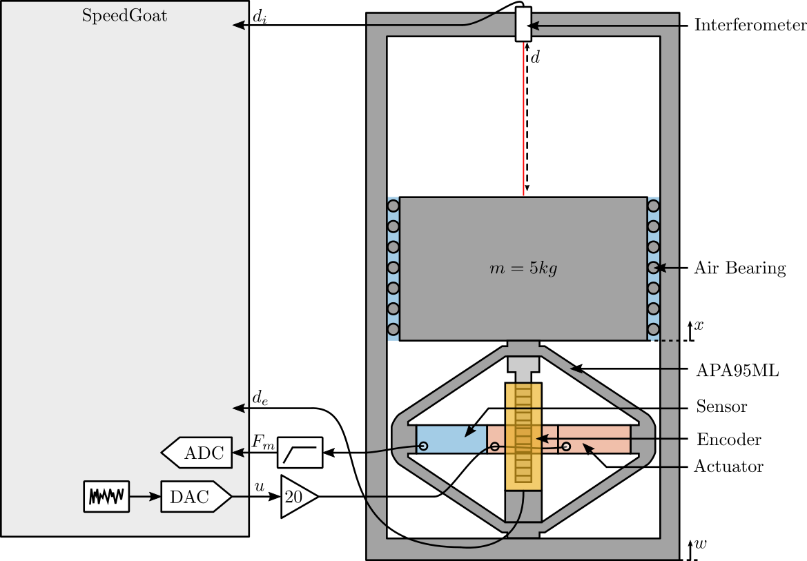
Figure 1: Schematic of the Experiment
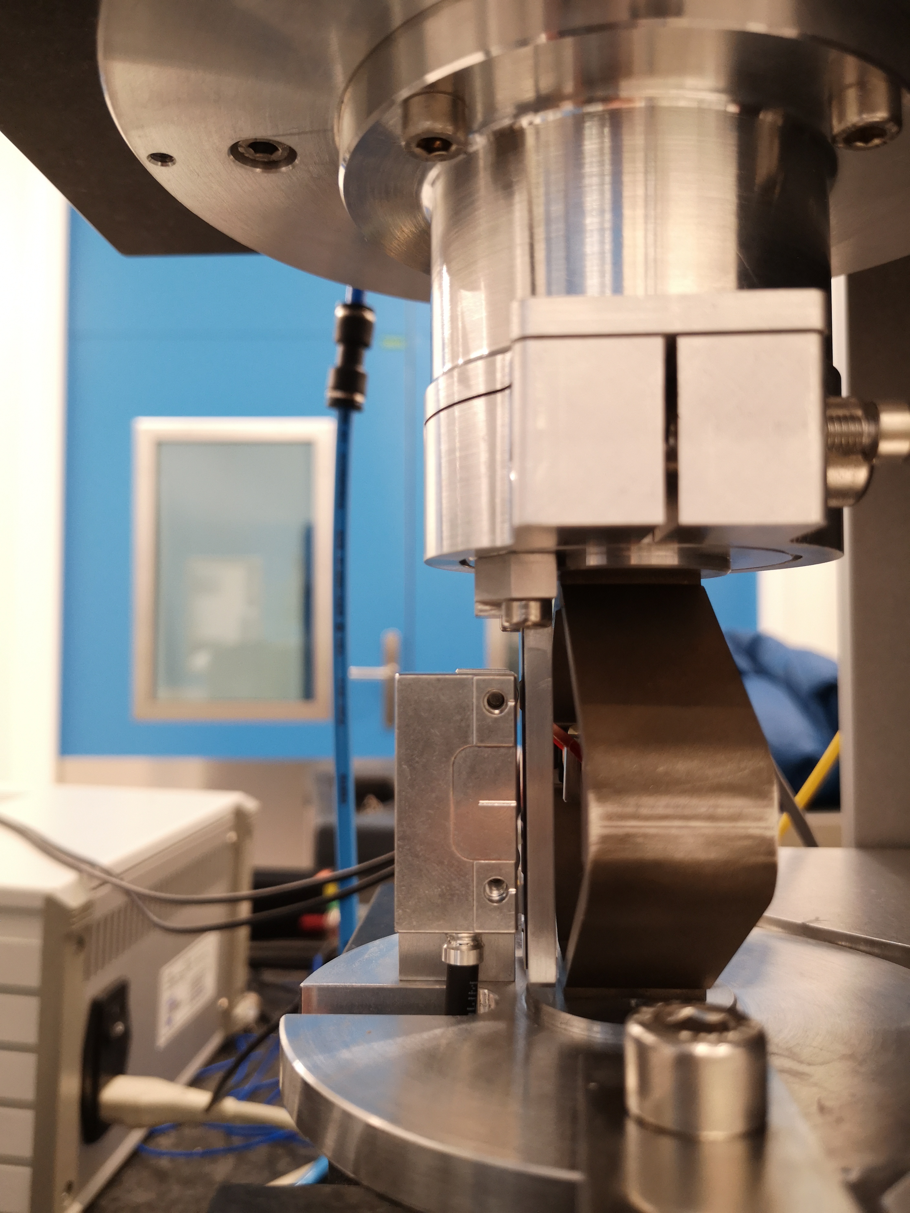
Figure 2: Side View of the encoder
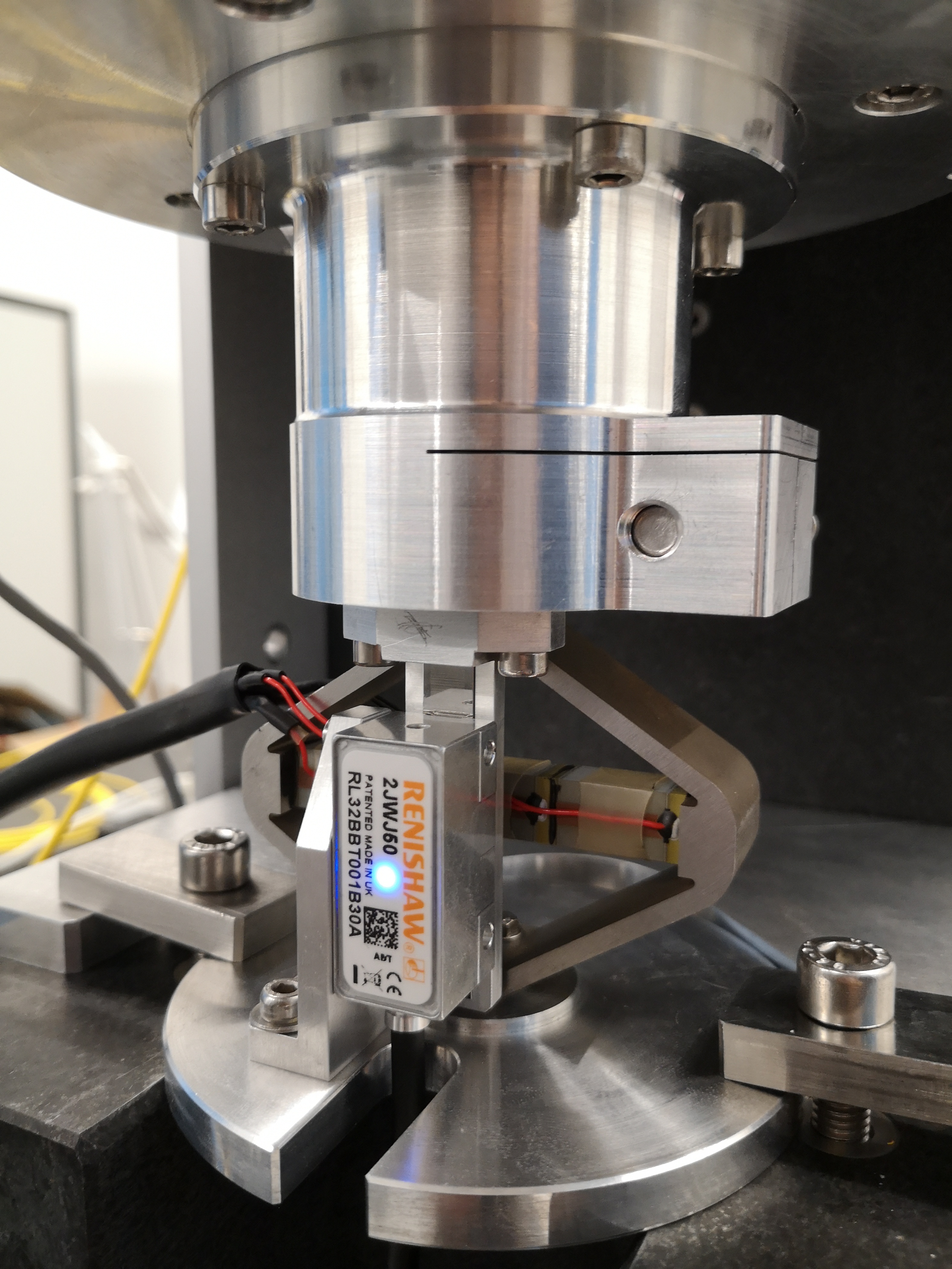
Figure 3: Front View of the encoder
2 Huddle Test
The goal in this section is the estimate the noise of both the encoder and the intereferometer.
Nothing is then to the actuator such that the relative motion between the mass and the frame is as small as possible. Ideally, a mechanical part would clamp the two together, we here suppose that the APA is still enough to clamp the two together.
2.1 Load Data
load('mat/int_enc_huddle_test.mat', 'interferometer', 'encoder', 't');
interferometer = detrend(interferometer, 0);
encoder = detrend(encoder, 0);
2.2 Time Domain Results
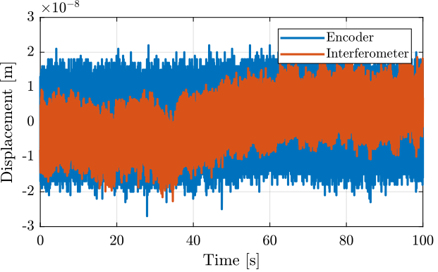
Figure 4: Huddle test - Time domain signals
G_lpf = 1/(1 + s/2/pi/10);
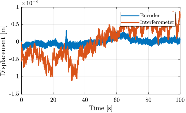
Figure 5: Huddle test - Time domain signals filtered with a LPF at 10Hz
2.3 Frequency Domain Noise
Ts = 1e-4;
win = hann(ceil(10/Ts));

[p_i, f] = pwelch(interferometer, win, [], [], 1/Ts);
[p_e, ~] = pwelch(encoder,        win, [], [], 1/Ts);
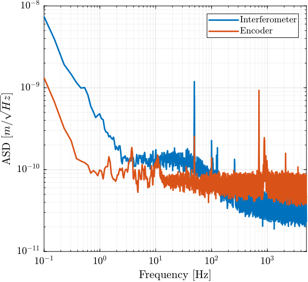
Figure 6: Amplitude Spectral Density of the signals during the Huddle test
3 Comparison Interferometer / Encoder
The goal here is to make sure that the interferometer and encoder measurements are coherent. We may see non-linearity in the interferometric measurement.
3.1 Load Data
load('mat/int_enc_comp.mat', 'interferometer', 'encoder', 'u', 't');
interferometer = detrend(interferometer, 0);
encoder = detrend(encoder, 0);
u = detrend(u, 0);
3.2 Time Domain Results
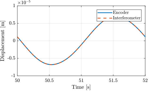
Figure 7: One cycle measurement
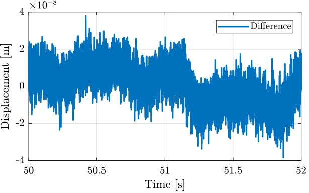
Figure 8: Difference between the Encoder and the interferometer during one cycle
3.3 Difference between Encoder and Interferometer as a function of time
Ts = 1e-4;
d_i_mean = reshape(interferometer, [2/Ts floor(Ts/2*length(interferometer))]);
d_e_mean = reshape(encoder,        [2/Ts floor(Ts/2*length(encoder))]);
w0 = 2*pi*5; % [rad/s]
xi = 0.7;

G_lpf = 1/(1 + 2*xi/w0*s + s^2/w0^2);

d_err_mean = reshape(lsim(G_lpf, encoder - interferometer, t), [2/Ts floor(Ts/2*length(encoder))]);
d_err_mean = d_err_mean - mean(d_err_mean);
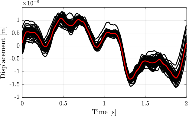
Figure 9: Difference between the two measurement in the time domain, averaged for all the cycles
3.4 Difference between Encoder and Interferometer as a function of position
Compute the mean of the interferometer measurement corresponding to each of the encoder measurement.
[e_sorted, ~, e_ind] = unique(encoder);

i_mean = zeros(length(e_sorted), 1);
for i = 1:length(e_sorted)
  i_mean(i) = mean(interferometer(e_ind == i));
end

i_mean_error = (i_mean - e_sorted);
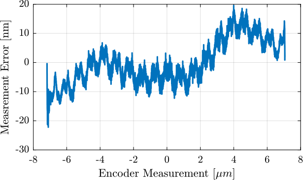
Figure 10: Difference between the two measurement as a function of the measured position by the encoder, averaged for all the cycles
The period of the non-linearity seems to be \(1.53 \mu m\) which corresponds to the wavelength of the Laser.
win_length = 1530; % length of the windows (corresponds to 1.53 um)
num_avg = floor(length(e_sorted)/win_length); % number of averaging

i_init = ceil((length(e_sorted) - win_length*num_avg)/2); % does not start at the extremity

e_sorted_mean_over_period = mean(reshape(i_mean_error(i_init:i_init+win_length*num_avg-1), [win_length num_avg]), 2);
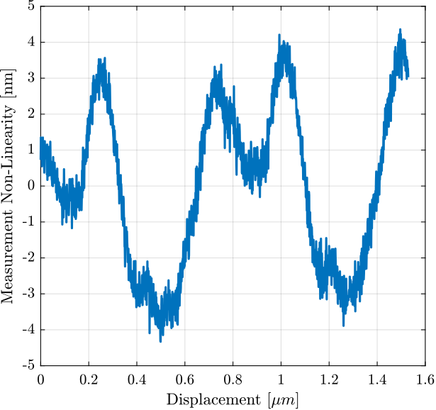
Figure 11: Non-Linearity of the Interferometer over the period of the wavelength
4 Identification
4.1 Load Data
load('mat/int_enc_id_noise_bis.mat', 'interferometer', 'encoder', 'u', 't');
interferometer = detrend(interferometer, 0);
encoder = detrend(encoder, 0);
u = detrend(u, 0);
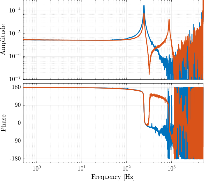
4.2 Identification
Ts = 1e-4; % Sampling Time [s]
win = hann(ceil(10/Ts));
[tf_i_est, f] = tfestimate(u, interferometer, win, [], [], 1/Ts);
[co_i_est, ~] = mscohere(u, interferometer, win, [], [], 1/Ts);

[tf_e_est, ~] = tfestimate(u, encoder, win, [], [], 1/Ts);
[co_e_est, ~] = mscohere(u, encoder, win, [], [], 1/Ts);
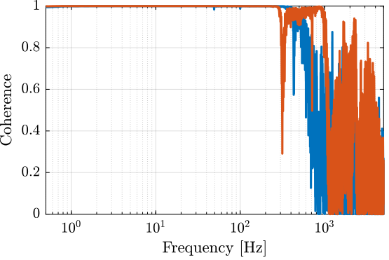
5 Change of Stiffness due to Sensors stack being open/closed circuit
5.1 Load Data
oc = load('./mat/identification_open_circuit.mat', 't', 'encoder', 'u');
sc = load('./mat/identification_short_circuit.mat', 't', 'encoder', 'u');
5.2 Transfer Functions
Ts = 1e-4; % Sampling Time [s]
win = hann(ceil(10/Ts));
[tf_oc_est, f] = tfestimate(oc.u, oc.encoder, win, [], [], 1/Ts);
[co_oc_est, ~] = mscohere(  oc.u, oc.encoder, win, [], [], 1/Ts);

[tf_sc_est, ~] = tfestimate(sc.u, sc.encoder, win, [], [], 1/Ts);
[co_sc_est, ~] = mscohere(  sc.u, sc.encoder, win, [], [], 1/Ts);
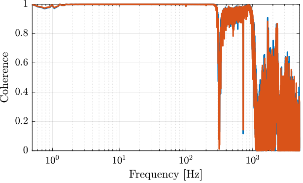
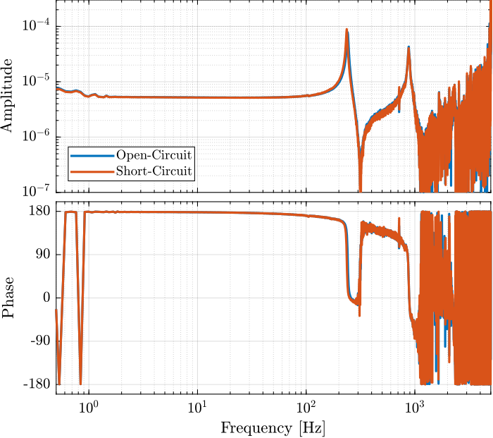
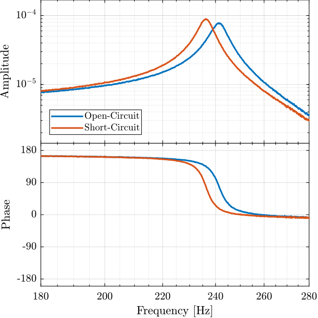
Figure 16: Zoom on the change of resonance
The change of resonance frequency / stiffness is very small and is not important here.
6 Generated Number of Charge / Voltage
Two stacks are used as actuator (in parallel) and one stack is used as sensor.
The amplifier gain is 20V/V (Cedrat LA75B).
6.1 Steps
load('./mat/force_sensor_steps.mat', 't', 'encoder', 'u', 'v');
figure;
tiledlayout(2, 1, 'TileSpacing', 'None', 'Padding', 'None');
nexttile;
plot(t, v);
xlabel('Time [s]'); ylabel('Measured voltage [V]');
nexttile;
plot(t, u);
xlabel('Time [s]'); ylabel('Actuator Voltage [V]');
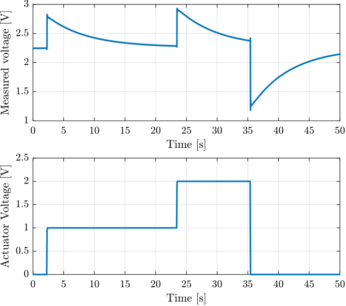
Figure 17: Time domain signal during the 3 actuator voltage steps
Three steps are performed at the following time intervals:
- 2.5, 23
- 23.8, 35
- 35.8, 50
Fit function:
f = @(b,x) b(1).*exp(b(2).*x) + b(3);
We are interested by the b(2) term, which is the time constant of the exponential.
tau = zeros(3,1);
V0  = zeros(3,1);
t_cur = t(2.5 < t & t < 23);
t_cur = t_cur - t_cur(1);
y_cur = v(2.5 < t & t < 23);

nrmrsd = @(b) norm(y_cur - f(b,t_cur)); % Residual Norm Cost Function
B0 = [0.5, -0.15, 2.2];                        % Choose Appropriate Initial Estimates
[B,rnrm] = fminsearch(nrmrsd, B0);     % Estimate Parameters ‘B’

tau(1) = 1/B(2);
V0(1)  = B(3);
t_cur = t(23.8 < t & t < 35);
t_cur = t_cur - t_cur(1);
y_cur = v(23.8 < t & t < 35);

nrmrsd = @(b) norm(y_cur - f(b,t_cur)); % Residual Norm Cost Function
B0 = [0.5, -0.15, 2.2];                 % Choose Appropriate Initial Estimates
[B,rnrm] = fminsearch(nrmrsd, B0);      % Estimate Parameters ‘B’

tau(2) = 1/B(2);
V0(2)  = B(3);
t_cur = t(35.8 < t);
t_cur = t_cur - t_cur(1);
y_cur = v(35.8 < t);

nrmrsd = @(b) norm(y_cur - f(b,t_cur)); % Residual Norm Cost Function
B0 = [0.5, -0.15, 2.2];                 % Choose Appropriate Initial Estimates
[B,rnrm] = fminsearch(nrmrsd, B0);     % Estimate Parameters ‘B’

tau(3) = 1/B(2);
V0(3)  = B(3);
| \(tau\) [s] | \(V_0\) [V] |
|---|---|
| 6.47 | 2.26 |
| 6.76 | 2.26 |
| 6.49 | 2.25 |
With the capacitance being \(C = 4.4 \mu F\), the internal impedance of the Speedgoat ADC can be computed as follows:
Cp = 4.4e-6; % [F]
Rin = abs(mean(tau))/Cp;
1494100.0
The input impedance of the Speedgoat’s ADC should then be close to \(1.5\,M\Omega\) (specified at \(1\,M\Omega\)).
How can we explain the voltage offset?
As shown in Figure 18 (taken from (Reza and Andrew 2006)), an input voltage offset is due to the input bias current \(i_n\).

Figure 18: Model of a piezoelectric transducer (left) and instrumentation amplifier (right)
The estimated input bias current is then:
in = mean(V0)/Rin;
1.5119e-06
An additional resistor in parallel with \(R_{in}\) would have two effects:
- reduce the input voltage offset \[ V_{off} = \frac{R_a R_{in}}{R_a + R_{in}} i_n \]
- increase the high pass corner frequency \(f_c\) \[ C_p \frac{R_{in}R_a}{R_{in} + R_a} = \tau_c = \frac{1}{f_c} \] \[ R_a = \frac{R_i}{f_c C_p R_i - 1} \]
If we allow the high pass corner frequency to be equals to 3Hz:
fc = 3;
Ra = Rin/(fc*C*Rin - 1);
79804
With this parallel resistance value, the voltage offset would be:
V_offset = Ra*Rin/(Ra + Rin) * in;
0.11454
Which is much more acceptable.
6.2 Sinus
load('./mat/force_sensor_sin.mat', 't', 'encoder', 'u', 'v');

u       = u(t>25);
v       = v(t>25);
encoder = encoder(t>25) - mean(encoder(t>25));
t       = t(t>25);
The driving voltage is a sinus at 0.5Hz centered on 3V and with an amplitude of 3V (Figure 19).
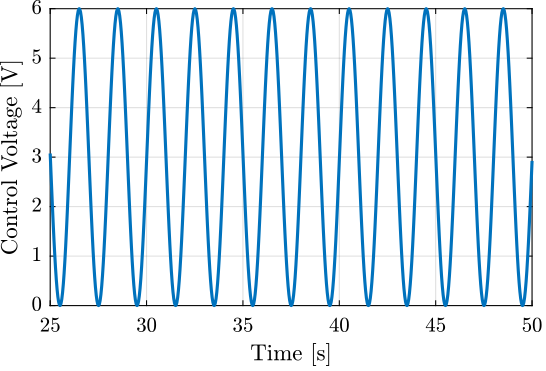
Figure 19: Driving Voltage
The full stroke as measured by the encoder is:
max(encoder)-min(encoder)
5.005e-05
Its signal is shown in Figure 20.
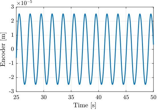
Figure 20: Encoder measurement
The generated voltage by the stack is shown in Figure
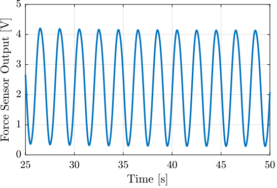
Figure 21: Voltage measured on the stack used as a sensor
The capacitance of the stack is
Cp = 4.4e-6; % [F]
The corresponding generated charge is then shown in Figure 22.
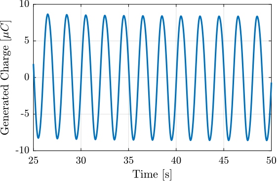
Figure 22: Generated Charge
The relation between the generated voltage and the measured displacement is almost linear as shown in Figure 23.
b1 = encoder\(v-mean(v));
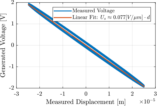
Figure 23: Almost linear relation between the relative displacement and the generated voltage
With a 16bits ADC, the resolution will then be equals to (in [nm]):
abs((20/2^16)/(b1/1e9))
3.9838