Encoder - Test Bench

1. Experimental Setup
2. Huddle Test
3. Comparison Interferometer / Encoder
4. Identification
- 4.1. Load Data
- 4.2. Identification

1 Experimental Setup

The experimental Setup is schematically represented in Figure 1.

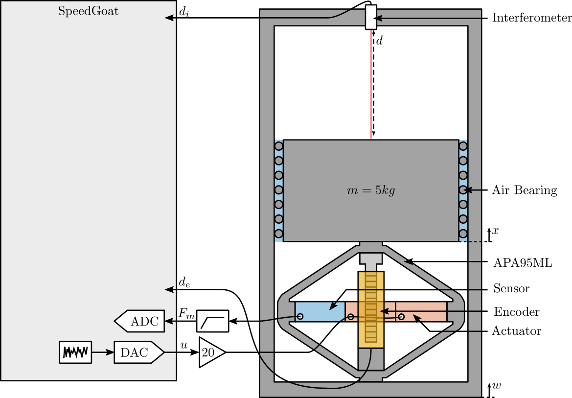
Figure 1: Schematic of the Experiment

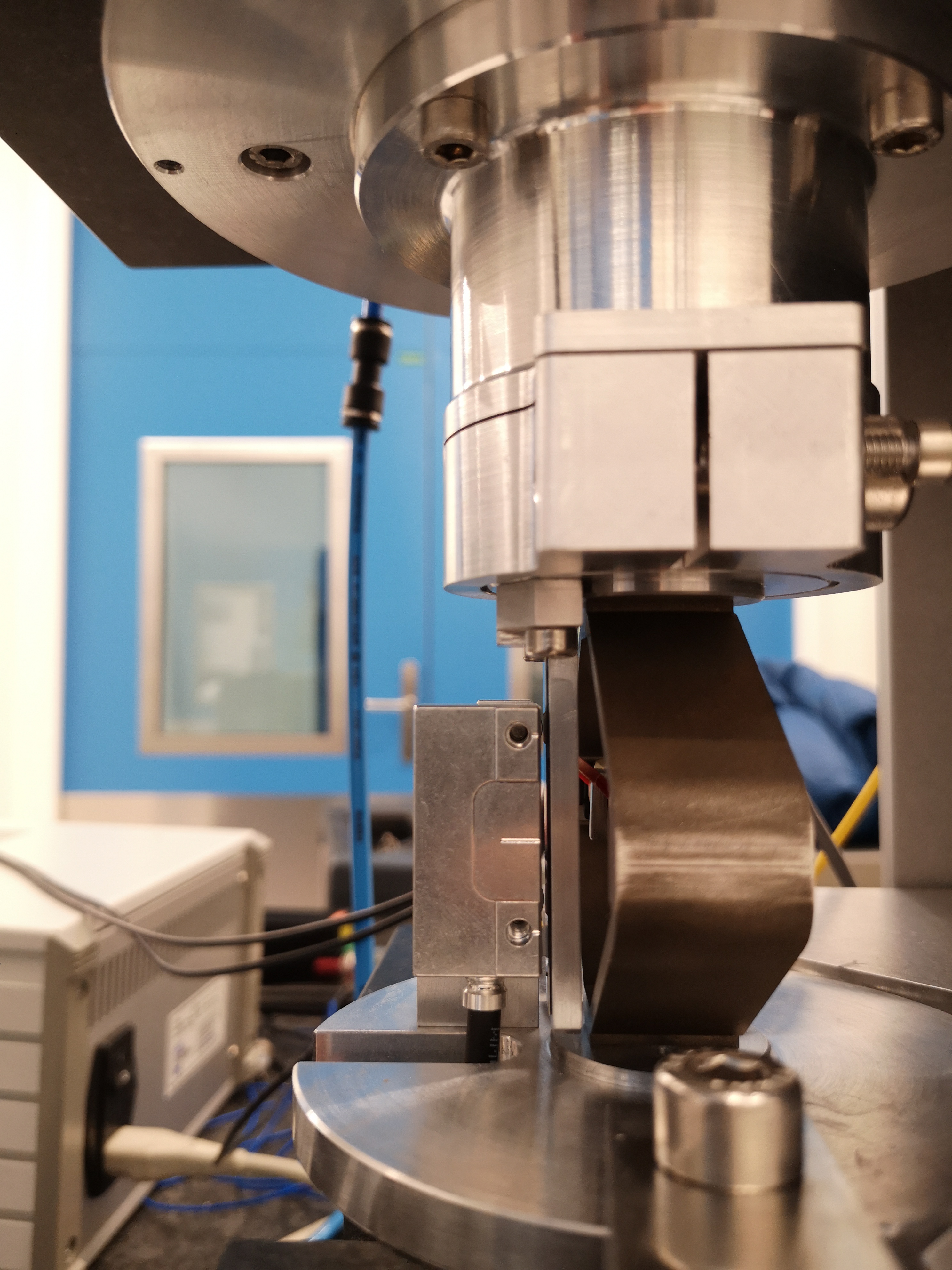
Figure 2: Side View of the encoder

Figure 3: Front View of the encoder

2 Huddle Test

The goal in this section is the estimate the noise of both the encoder and the intereferometer.

2.1 Load Data

load('mat/int_enc_huddle_test.mat', 'interferometer', 'encoder', 't');

interferometer = detrend(interferometer, 0);
encoder = detrend(encoder, 0);

2.2 Time Domain Results

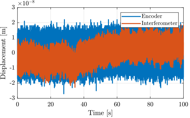
Figure 4: Huddle test - Time domain signals

G_lpf = 1/(1 + s/2/pi/10);

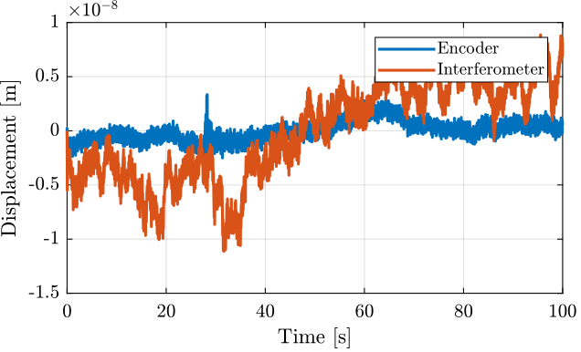
Figure 5: Huddle test - Time domain signals filtered with a LPF at 10Hz

2.3 Frequency Domain Noise

Ts = 1e-4;
win = hann(ceil(10/Ts));

[p_i, f] = pwelch(interferometer, win, [], [], 1/Ts);
[p_e, ~] = pwelch(encoder,        win, [], [], 1/Ts);

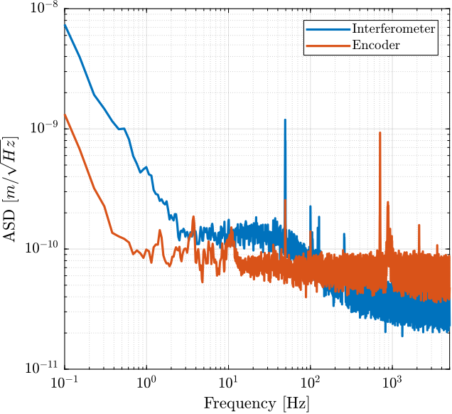
Figure 6: Amplitude Spectral Density of the signals during the Huddle test

3 Comparison Interferometer / Encoder

The goal here is to make sure that the interferometer and encoder measurements are coherent. We may see non-linearity in the interferometric measurement.

3.1 Load Data

load('mat/int_enc_comp.mat', 'interferometer', 'encoder', 'u', 't');

interferometer = detrend(interferometer, 0);
encoder = detrend(encoder, 0);
u = detrend(u, 0);

3.2 Time Domain Results

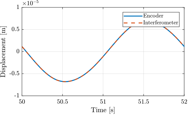
Figure 7: One cycle measurement

Figure 8: Difference between the Encoder and the interferometer during one cycle

3.3 Difference between Encoder and Interferometer as a function of time

Ts = 1e-4;
d_i_mean = reshape(interferometer, [2/Ts floor(Ts/2*length(interferometer))]);
d_e_mean = reshape(encoder,        [2/Ts floor(Ts/2*length(encoder))]);

w0 = 2*pi*5; % [rad/s]
xi = 0.7;

G_lpf = 1/(1 + 2*xi/w0*s + s^2/w0^2);

d_err_mean = reshape(lsim(G_lpf, encoder - interferometer, t), [2/Ts floor(Ts/2*length(encoder))]);
d_err_mean = d_err_mean - mean(d_err_mean);

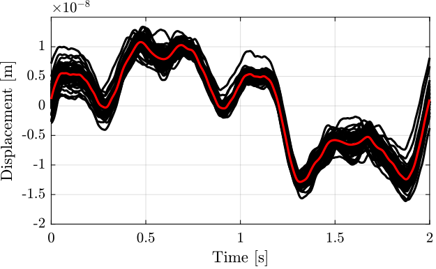
Figure 9: Difference between the two measurement in the time domain, averaged for all the cycles

3.4 Difference between Encoder and Interferometer as a function of position

Compute the mean of the interferometer measurement corresponding to each of the encoder measurement.

[e_sorted, ~, e_ind] = unique(encoder);

i_mean = zeros(length(e_sorted), 1);
for i = 1:length(e_sorted)
  i_mean(i) = mean(interferometer(e_ind == i));
end

i_mean_error = (i_mean - e_sorted);

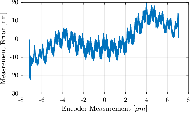
Figure 10: Difference between the two measurement as a function of the measured position by the encoder, averaged for all the cycles

The period of the non-linearity seems to be \(1.53 \mu m\) which corresponds to the wavelength of the Laser.

win_length = 1530; % length of the windows (corresponds to 1.53 um)
num_avg = floor(length(e_sorted)/win_length); % number of averaging

i_init = ceil((length(e_sorted) - win_length*num_avg)/2); % does not start at the extremity

e_sorted_mean_over_period = mean(reshape(i_mean_error(i_init:i_init+win_length*num_avg-1), [win_length num_avg]), 2);

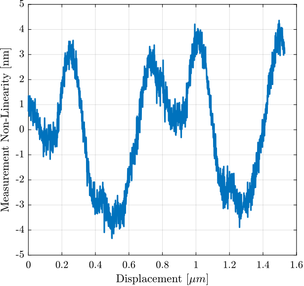
Figure 11: Non-Linearity of the Interferometer over the period of the wavelength

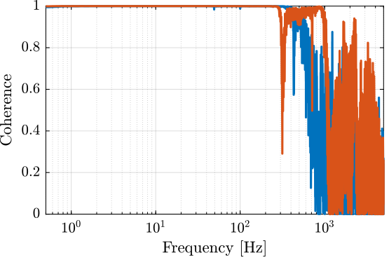
4 Identification

4.1 Load Data

load('mat/int_enc_id_noise_bis.mat', 'interferometer', 'encoder', 'u', 't');

interferometer = detrend(interferometer, 0);
encoder = detrend(encoder, 0);
u = detrend(u, 0);

4.2 Identification

Ts = 1e-4; % Sampling Time [s]
win = hann(ceil(10/Ts));

[tf_i_est, f] = tfestimate(u, interferometer, win, [], [], 1/Ts);
[co_i_est, ~] = mscohere(u, interferometer, win, [], [], 1/Ts);

[tf_e_est, ~] = tfestimate(u, encoder, win, [], [], 1/Ts);
[co_e_est, ~] = mscohere(u, encoder, win, [], [], 1/Ts);