Delta Robot

1. Studied Geometry
2. Kinematics: Jacobian Matrix and Mobility
3. Kinematics: Degrees of Freedom
4. Kinematics: Number of modes
5. Flexible Joint Design
6. Effect of the Geometry
7. Conclusion

1. Studied Geometry

The Delta Robot geometry is defined as shown in Figure 1.

The geometry is fully defined by three parameters:

d: Cube’s size (i.e., the length of the cube edge)
a: Distance from cube’s vertex to top flexible joint
L: Distance between two flexible joints (i.e., the length of the struts)

Figure 1: Schematic of the Delta Robot

Several frames are defined:

\(\{C\}\): Cube’s center
\(\{M\}\): Frame attached to the mobile platform, and located at the height of the top flexible joints
\(\{F\}\): Frame attached to the fixed platform, and located at the height of the bottom flexible joints

Several points are defined:

\(c_i\): vertices of the cubes which are relevant for the Delta Robot
\(b_i\): location of the top flexible joints
\(a_i\): location of the bottom flexible joints
\(\hat{s}_i\): unit vector aligned with the struts

Static properties:

All top and bottom flexible joints are identical. The following properties can be specified:
- \(k_a\): Axial stiffness
- \(k_r\): Radial stiffness
- \(k_b\): Bending stiffness
- \(k_t\): Torsion stiffness
The guiding mechanism of the actuator is here supposed to be perfect (i.e. 1dof system without any stiffness)
The Actuator is modelled as a 1DoF or 2DoF (good to model APA):
- The custom developed APA has an axial stiffness of \(1.3\,N/\mu m\)

Dynamical properties:

Top platform inertia: It has a mass of ~300g
Payloads: payloads can weight up to 1kg

Let’s initialize a Delta Robot architecture, and plot the obtained geometry (Figures 2 and 3).

%% Geometry
d = 50e-3; % Cube's edge length [m]
b = 20e-3; % Distance between cube's vertices and top joints [m]
L = 50e-3; % Length of the struts [m]

Figure 2: Delta Robot Architecture

Figure 3: Delta Robot Architecture - Top View

2. Kinematics: Jacobian Matrix and Mobility

There are three actuators in the following directions \(\hat{s}_1\), \(\hat{s}_2\) and \(\hat{s}_3\);

\begin{equation}\label{eq:delta_robot_unit_vectors} \hat{\bm{s}}_1 = \begin{bmatrix} \frac{-1}{\sqrt{6}} \\ \frac{-1}{\sqrt{2}} \\ \frac{1}{\sqrt{3}} \end{bmatrix}\quad \hat{\bm{s}}_2 = \begin{bmatrix} \frac{\sqrt{2}}{\sqrt{3}} \\ 0 \\ \frac{1}{\sqrt{3}} \end{bmatrix}\quad \hat{\bm{s}}_3 = \begin{bmatrix} \frac{-1}{\sqrt{6}} \\ \frac{ 1}{\sqrt{2}} \\ \frac{1}{\sqrt{3}} \end{bmatrix} \end{equation}

The Jacobian matrix is defined as shown in \ref{eq:delta_robot_jacobian}.

\begin{equation}\label{eq:delta_robot_jacobian} \bm{J} = \begin{bmatrix} \hat{\bm{s}}_1^T \\ \hat{\bm{s}}_2^T \\ \hat{\bm{s}}_3^T \end{bmatrix} \end{equation}

It links the small actuator displacement to the top platform displacement \ref{eq:delta_robot_inverse_kinematics}.

\begin{equation}\label{eq:delta_robot_inverse_kinematics} d\mathcal{L} = J d\mathcal{L} \end{equation} \begin{equation}\label{eq:delta_robot_forward_kinematics} d\mathcal{X} = J^{-1} d\mathcal{L} \end{equation}

The achievable workspace is a cube whose edge length is equal to the actuator stroke.

Figure 4: 3D workspace

As most likely, the system will be used to perform YZ scans, it is interesting to see the mobility of the system in the ZY plane.

Depending on how the YZ plane is oriented (i.e., depending on the Rz angle of the delta robot with respect to the beam, defining the x direction), we get different mobility.

Figure 5: 2D mobility for different orientations and worst case

Maximum YZ mobility for an angle of 270 degrees, square with edge size of 117 um

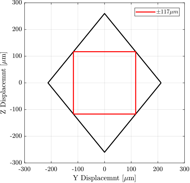
Figure 6: 2D mobility for the optimal Rz angle

3. Kinematics: Degrees of Freedom

In the perfect case (flexible joints having no stiffness in bending, and infinite stiffness in torsion and in the axial direction), the top platform is allowed to move only in the X, Y and Z directions while the three rotations are fixed.

In order to have some compliance in rotation, the flexible joints need to have some compliance in torsion and in the axial direction. If only the torsional compliance is considered, or only the axial compliance, the top platform will still not be able to do any rotation.

This is shown below with the Simscape model.

Perfect Delta Robot:

infinite axial stiffness
infinite torsional stiffness
no bending stiffness

It gives infinite stiffness in rotations, and a stiffness of \(1\,N/\mu m\) in X, Y and Z directions (i.e. equal to the actuator stiffness).

Stiffness in X,Y and Z directions: 1.0 N/um

If we consider the torsion of the flexible joints:

infinite axial stiffness
finite torsional stiffness
no bending stiffness

We get the same result.

If we consider the axial of the flexible joints:

finite axial stiffness
infinite torsional stiffness
no bending stiffness

We get the same result.

No we consider both finite torsional stiffness and finite axial stiffness. In that case we get some compliance in rotation. So it is a combination of axial and torsion stiffness that gives some rotational stiffness of the top platform.

Therefore, to model some compliance of the top platform in rotation, both the axial compliance and the torsional compliance of the flexible joints should be considered.

4. Kinematics: Number of modes

In the perfect condition (i.e. infinite stiffness in torsion and in compression of the flexible joints), the system has 6 states (i.e. 3 modes, one for each DoF: X, Y and Z).

When considering some compliance in torsion of the flexible joints, 12 states are added (one internal mode of the struts). To remove these internal states (that might not be interesting but that could slow the simulations), one of the joint can have this torsional compliance while the other can have the torsional DoF constrained.

State-space model with 3 outputs, 3 inputs, and 6 states.

5. Flexible Joint Design

First, in Section 5.1, the dynamics of a “perfect” Delta-Robot is identified (i.e. with perfect 2DoF rotational joints).

Then, the impact of the flexible joint’s imperfections will be studied. The goal is to extract specifications for the flexible joints of the six struts, in terms of:

bending stiffness (Section 5.2)
axial stiffness (Section 5.3)
torsional stiffness (Section 5.4)
shear stiffness (Section 5.5)

5.1. Studied Geometry

The cube’s edge length is equal to 50mm, the distance between cube’s vertices and top joints is 20mm and the length of the struts (i.e. the distance between the two flexible joints of the same strut) is 50mm. The actuator stiffness is \(1\,N/\mu m\).

The obtained geometry is shown in Figure [].

Figure 7: Geometry of the studied Delta Robot

The dynamics is first identified in perfect conditions (infinite axial stiffness of the joints, zero bending stiffness). We get State-space model with 3 outputs, 3 inputs, and 6 states. We get a perfectly decoupled system, with three identical modes in the X, Y and Z directions. The dynamics is shown in Figure 8.

Figure 8: Dynamics of the delta robot with perfect joints

5.2. Bending Stiffness

5.2.1. Stiffness seen by the actuator, and decrease of the achievable stroke

Because the flexible joints will have some bending stiffness, the actuator in one direction will “see” some stiffness due to the struts in the other directions. This will limit its effective stroke. We want this parallel stiffness to be much smaller than the stiffness of the actuator.

The parallel stiffness seen by the actuator as a function of the bending stiffness of the flexible joints is computed and shown in Figure 9.

Figure 9: Effect of the bending stiffness of the flexible joints on the stiffness seen by the actuators

The parallel stiffness is therefore proportional to the bending stiffness. The “linear coefficient” depend on the geometry, and it is here equal to \(3200 \frac{N/m}{Nm/\text{rad}}\).

If we want the parallel stiffness to be much smaller than the stiffness of the actuator (\(k_p \ll k_a = 1.6\,N/\mu m\)), the bending stiffness should be \(\ll 500\,Nm/\text{rad}\). Therefore, we should aim at \(k_f < 50\,Nm/\text{rad}\).

This should be validated with the final geometry.

Then, the dynamics is identified for a bending Stiffness of \(50\,Nm/\text{rad}\) and compared with a Delta robot with no bending stiffness in Figure 10.

It can be seen that the DC gain is a bit lower when the bending stiffness is considered and the resonance frequency is increased. This simply means that the system stiffness is increased. It is not critical from a dynamical point of view, it just decreases the achievable stroke as explained in the previous section.

Figure 10: Effect of the bending stiffness on the dynamics

5.2.2. Effect on the coupling

Here, reasonable values for the flexible joints (modelled as a 6DoF joint) stiffness are taken:

Torsional stiffness of 500Nm/rad
Axial stiffness of 100N/um
Shear stiffness of 100N/um

And the bending stiffness is varied from low to high values. The obtained dynamics is shown in Figure 11. It can be seen that the low frequency coupling increases when the bending stiffness increases.

Therefore, the bending stiffness of the flexible joints should be minimized (10Nm/rad could be a reasonable objective).

Figure 11: Effect of the bending stiffness of the flexible joints on the coupling

5.3. Axial Stiffness

Now, the effect of the axial stiffness on the dynamics is studied (Figure 12). Additional modes can be observed on the plant dynamics, which could limit the achievable bandwidth. Therefore the axial stiffness should be maximized. Having the axial stiffness 100 times stiffer than the actuator stiffness seems reasonable. Therefore, we should aim at \(k_a > 100\,N/\mu m\).

Figure 12: Effect of the joint’s axial stiffness on the plant dynamics

5.4. Torsional Stiffness

Now the compliance in torsion of the flexible joints is considered.

If we look at the compliance of the delta robot in rotation as a function of the torsional stiffness of the flexible joints (Figure 13), we see almost no effect: the system is not made more stiff by increasing the torsional stiffness of the joints.

Figure 13: Effect of the joint’s torsional stiffness on the Delta Robot compliance

If we have a look at the effect of the torsional stiffness on the plant dynamics (Figure 14), we see almost no effect, except when super high values are reached (\(10^6\,Nm/\text{rad}\)), which are unrealistic.

Figure 14: Effect of the joint’s torsional stiffness on the Delta Robot plant dynamics

Therefore, the torsional stiffness is not a super important metric for the design of the delta robot.

5.5. Shear Stiffness

As shown in Figure 15, the shear stiffness of the flexible joints has some effect on the compliance in translation and almost no effect on the compliance in rotation.

This is quite logical, and so the shear stiffness should be maximized. A value of \(100\,N/\mu m\) seems reasonable.

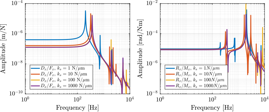
Figure 15: Effect of the shear stiffness of the flexible joints on the Delta Robot compliance

5.6. Conclusion

Table 1: Recommendations for the flexible joints
Joint’s Stiffness	Effect	Recommendation
Bending	Can reduce the stroke, and increase the coupling	Below 50 to 10 Nm/rad
Axial	Add modes that can limit the feedback bandwidth	As high as possible, at least 100 Nm/um
Torsion	Minor effect	No recommendation
Shear	Can limit the stiffness of the system	As high as possible (less important than the axial stiffness), above 100 N/um if possible

6. Effect of the Geometry

6.1. Effect of cube’s size

Let’s choose reasonable values for the flexible joints:

Bending stiffness of 50Nm/rad
Torsional stiffness of 500Nm/rad
Axial stiffness of 100N/um
Shear stiffness of 100N/um

And we see the effect of changing the cube’s size.

6.1.1. Effect on the plant dynamics

[ ] Understand why such different dynamics between 3dof_a joints and 6dof joints with very high shear stiffnesses

The effect of the cube’s size on the plant dynamics is shown in Figure 16:

coupling decreases with the cube’s size
one resonance frequency increases with the cube’s size (resonances in rotation), which may be beneficial from a control point of view
coupling at the main resonance varies with the cube’s size, but it may also depend on the relative position between the CoM and the cube’s center

Figure 16: Effect of the cube’s size on the plant dynamics

6.1.2. Effect on the compliance

As shown in Figure 17, the stiffness of the delta robot in rotation increases with the cube’s size.

Figure 17: Effect of the cube’s size on the rotational compliance of the top platform

With a cube size of 50mm, the resonance frequency is already above 1kHz with seems reasonable.

6.2. Effect of the strut length

Let’s choose reasonable values for the flexible joints:

Bending stiffness of 50Nm/rad
Torsional stiffness of 500Nm/rad
Axial stiffness of 100N/um

And we see the effect of changing the strut length.

6.2.1. Effect on the compliance

As shown in Figure 18, the strut length has an effect on the system stiffness in translation (left plot) but almost not in rotation (right plot).

Indeed, the stiffness in rotation is a combination of:

The stiffness of the actuator
The shear and axial stiffness of the flexible joints
The bending and torsional stiffness of the flexible joints, combine with the strut length

Figure 18: Effect of the cube’s size on the rotational compliance of the top platform

6.2.2. Effect on the plant dynamics

As shown in Figure 19, having longer struts:

decreases the main resonance frequency: this means that the stiffness in the X,Y and Z directions is decreased when the length of the strut is longer. This is reasonable as the “lever” arm is getting larger, so the bending stiffness and compression of the flexible joints have a larger effect on the top platform compliance.
decreases the low frequency coupling: this effect is more difficult to physically understand Probably: when pushing with one actuator, it induces some rotation of the struts corresponding to the other two actuators. This rotation is proportional to the strut length. Then, this rotation, combined with the limited compliance in bending of the flexible joints induces some force applied on the other actuators, hence the coupling. This is similar to what was observed when varying the bending stiffness of the flexible joints: the coupling was increased with an increased of the bending stiffness (See Figure 11) So we should also observed a decrease of the coupling when decreasing the bending stiffness of the actuators

But even with relatively short struts (20mm and above), the low frequency decoupling is already around two orders of magnitude, which is enough from a control point of view. So, the struts length can be optimized to not decrease too much the stiffness of the platform while still getting good low frequency decoupling.

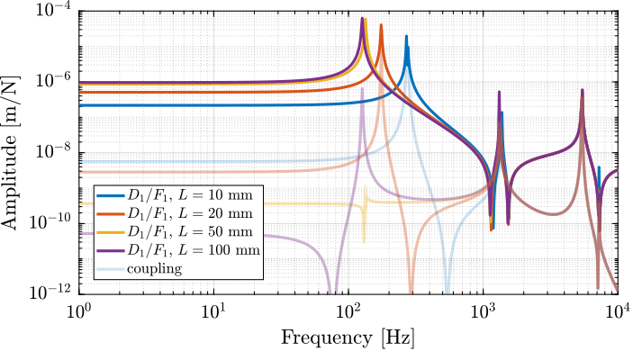
Figure 19: Effect of the Strut length on the plant dynamics

6.3. Having the Center of Mass at the cube’s center

To make things easier, we take a top platform with no mass, mass-less struts, and we put a payload on top of the platform.

As shown in Figure 20, having the CoM of the payload at the cube’s center allow to have better decoupling properties above the suspension mode of the system (i.e. above the first mode). This could allow to have a bandwidth exceeding the frequency of the first mode. But how sensitive this decoupling is to the exact position of the CoM still need to be studied.

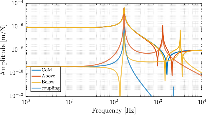
Figure 20: Effect of the payload’s Center of Mass position with respect to the cube’s size on the plant dynamics