A new method of designing complementary filters for sensor fusion using the \(\mathcal{H}_\infty\) synthesis - Matlab Computation

1. H-Infinity synthesis of complementary filters
2. Design of complementary filters used in the Active Vibration Isolation System at the LIGO
3. “Closed-Loop” complementary filters
4. Synthesis of three complementary filters
5. Matlab Scripts

This report is also available as a pdf.

The present document is a companion file for the journal paper (Dehaeze, Vermat, and Collette 2004). All the Matlab (MATLAB 2020) scripts used in the paper are here shared and explained.

This document is divided into the following sections also corresponding to the paper sections:

Section 1: the shaping of complementary filters is written as an \(\mathcal{H}_\infty\) optimization problem using weighting functions. The weighting function design is discussed and the method is applied for the design of a set of simple complementary filters.
Section 2: the effectiveness of the proposed complementary filter synthesis strategy is demonstrated by designing complex complementary filters used in the first isolation stage at the LIGO
Section 3: complementary filters are designed using the classical feedback loop
Section 4: the proposed design method is generalized for the design of a set of three complementary filters
Section 5: complete Matlab scripts and functions developed are listed

1. H-Infinity synthesis of complementary filters

1.1. Synthesis Architecture

In order to generate two complementary filters with a wanted shape, the generalized plant of Figure 1 can be used. The included weights \(W_1(s)\) and \(W_2(s)\) are used to specify the upper bounds of the complementary filters being generated.

Figure 1: Generalized plant used for the \(\mathcal{H}_\infty\) synthesis of a set of two complementary fiters

Applied the standard \(\mathcal{H}_\infty\) synthesis on this generalized plant will give a transfer function \(H_2(s)\) (see Figure 2) such that the \(\mathcal{H}_\infty\) norm of the transfer function from \(w\) to \([z_1,\ z_2]\) is less than one \eqref{eq:h_inf_objective}.

Figure 2: Generalized plant with the synthesized filter obtained after the \(\mathcal{H}_\infty\) synthesis

\begin{equation} \left\| \begin{array}{c} (1 - H_2(s)) W_1(s) \\ H_2(s) W_2(s) \end{array} \right\|_\infty < 1 \label{eq:h_inf_objective} \end{equation}

Thus, if the synthesis is successful and the above condition is verified, we can define \(H_1(s)\) to be the complementary of \(H_2(s)\) \eqref{eq:H1_complementary_of_H2} and we have condition \eqref{eq:shaping_comp_filters} verified.

\begin{equation} H_1(s) = 1 - H_2(s) \label{eq:H1_complementary_of_H2} \end{equation} \begin{equation} \left\| \begin{array}{c} H_1(s) W_1(s) \\ H_2(s) W_2(s) \end{array} \right\|_\infty < 1 \quad \Longrightarrow \quad \left\{ \begin{array}{c} |H_1(j\omega)| < \frac{1}{|W_1(j\omega)|}, \quad \forall \omega \\ |H_2(j\omega)| < \frac{1}{|W_2(j\omega)|}, \quad \forall \omega \end{array} \right. \label{eq:shaping_comp_filters} \end{equation}

We then see that \(W_1(s)\) and \(W_2(s)\) can be used to set the wanted upper bounds of the magnitudes of both \(H_1(s)\) and \(H_2(s)\).

The presented synthesis method therefore allows to shape two filters \(H_1(s)\) and \(H_2(s)\) \eqref{eq:shaping_comp_filters} while ensuring their complementary property \eqref{eq:H1_complementary_of_H2}.

The complete Matlab script for this part is given in Section 5.1.

1.2. Design of Weighting Function - Proposed formula

A formula is proposed to help the design of the weighting functions:

\begin{equation} W(s) = \left( \frac{ \frac{1}{\omega_0} \sqrt{\frac{1 - \left(\frac{G_0}{G_c}\right)^{\frac{2}{n}}}{1 - \left(\frac{G_c}{G_\infty}\right)^{\frac{2}{n}}}} s + \left(\frac{G_0}{G_c}\right)^{\frac{1}{n}} }{ \left(\frac{1}{G_\infty}\right)^{\frac{1}{n}} \frac{1}{\omega_0} \sqrt{\frac{1 - \left(\frac{G_0}{G_c}\right)^{\frac{2}{n}}}{1 - \left(\frac{G_c}{G_\infty}\right)^{\frac{2}{n}}}} s + \left(\frac{1}{G_c}\right)^{\frac{1}{n}} }\right)^n \label{eq:weighting_function_formula} \end{equation}

The parameters permits to specify:

the low frequency gain: \(G_0 = lim_{\omega \to 0} |W(j\omega)|\)
the high frequency gain: \(G_\infty = lim_{\omega \to \infty} |W(j\omega)|\)
the absolute gain at \(\omega_0\): \(G_c = |W(j\omega_0)|\)
the absolute slope between high and low frequency: \(n\)

The general shape of a weighting function generated using the formula is shown in figure 3.

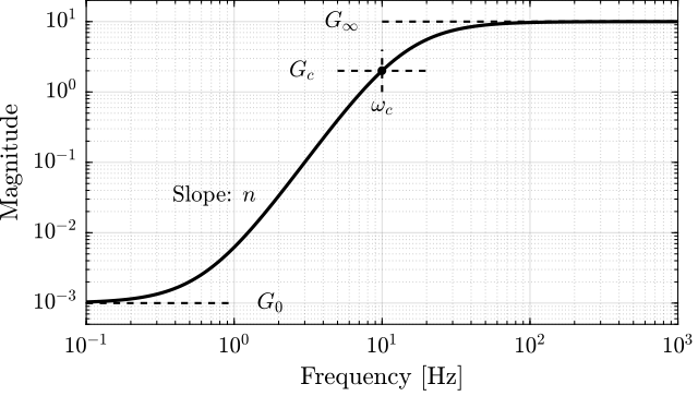
Figure 3: Magnitude of the weighting function generated using formula \eqref{eq:weighting_function_formula}

1.3. Weighting functions for the design of two complementary filters

The weighting function formula \eqref{eq:weighting_function_formula} is used to generate the upper bounds of two complementary filters that we wish to design.

The matlab function generateWF is described in Section 5.5.

%% Design of the Weighting Functions
W1 = generateWF('n', 3, 'w0', 2*pi*10, 'G0', 1000, 'Ginf', 1/10, 'Gc', 0.45);
W2 = generateWF('n', 2, 'w0', 2*pi*10, 'G0', 1/10, 'Ginf', 1000, 'Gc', 0.45);

The inverse magnitude of these two weighting functions are shown in Figure 4.

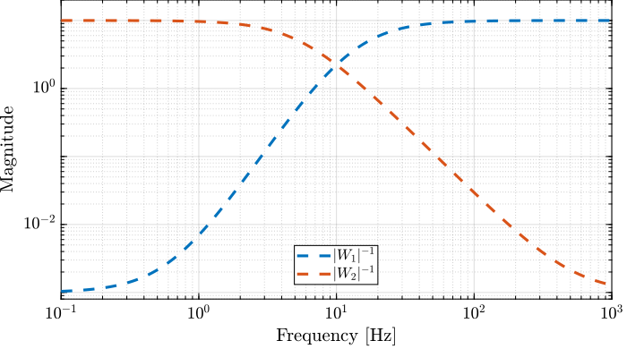
Figure 4: Inverse magnitude of the design weighting functions

1.4. Synthesis of the complementary filters

The generalized plant of Figure 1 is defined as follows:

%% Generalized Plant
P = [W1 -W1;
     0   W2;
     1   0];

And the \(\mathcal{H}_\infty\) synthesis is performed using the hinfsyn command.

%% H-Infinity Synthesis
[H2, ~, gamma, ~] = hinfsyn(P, 1, 1,'TOLGAM', 0.001, 'METHOD', 'ric', 'DISPLAY', 'on');

[H2, ~, gamma, ~] = hinfsyn(P, 1, 1,'TOLGAM', 0.001, 'METHOD', 'ric', 'DISPLAY', 'on');

  Test bounds:  0.3223 <=  gamma  <=  1000

    gamma        X>=0        Y>=0       rho(XY)<1    p/f
  1.795e+01     1.4e-07     0.0e+00     1.481e-16     p
  2.406e+00     1.4e-07     0.0e+00     3.604e-15     p
  8.806e-01    -3.1e+02 #  -1.4e-16     7.370e-19     f
  1.456e+00     1.4e-07     0.0e+00     1.499e-18     p
  1.132e+00     1.4e-07     0.0e+00     8.587e-15     p
  9.985e-01     1.4e-07     0.0e+00     2.331e-13     p
  9.377e-01    -7.7e+02 #  -6.6e-17     3.744e-14     f
  9.676e-01    -2.0e+03 #  -5.7e-17     1.046e-13     f
  9.829e-01    -6.6e+03 #  -1.1e-16     2.949e-13     f
  9.907e-01     1.4e-07     0.0e+00     2.374e-19     p
  9.868e-01    -1.6e+04 #  -6.4e-17     5.331e-14     f
  9.887e-01    -5.1e+04 #  -1.5e-17     2.703e-19     f
  9.897e-01     1.4e-07     0.0e+00     1.583e-11     p
  Limiting gains...
  9.897e-01     1.5e-07     0.0e+00     1.183e-12     p
  9.897e-01     6.9e-07     0.0e+00     1.365e-12     p

  Best performance (actual): 0.9897

As shown above, the obtained \(\mathcal{H}_\infty\) norm of the transfer function from \(w\) to \([z_1,\ z_2]\) is found to be less than one meaning the synthesis is successful.

We then define the filter \(H_1(s)\) to be the complementary of \(H_2(s)\) \eqref{eq:H1_complementary_of_H2}.

%% Define H1 to be the complementary of H2
H1 = 1 - H2;

The function generateCF can also be used to synthesize the complementary filters. This function is described in Section 5.6.

[H1, H2] = generateCF(W1, W2);

1.5. Obtained Complementary Filters

The obtained complementary filters are shown below and are found to be of order 5. Their bode plots are shown in figure 5 and compare with the defined upper bounds.

zpk(H1)
ans =

            (s+1.289e05) (s+153.6) (s+3.842)^3
  -------------------------------------------------------
  (s+1.29e05) (s^2 + 102.1s + 2733) (s^2 + 69.45s + 3272)

zpk(H2)
ans =

         125.61 (s+3358)^2 (s^2 + 46.61s + 813.8)
  -------------------------------------------------------
  (s+1.29e05) (s^2 + 102.1s + 2733) (s^2 + 69.45s + 3272)

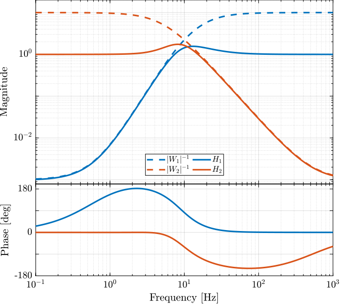
Figure 5: Obtained complementary filters using \(\mathcal{H}_\infty\) synthesis

2. Design of complementary filters used in the Active Vibration Isolation System at the LIGO

In this section, the proposed method for the design of complementary filters is validated for the design of a set of two complex complementary filters used for the first isolation stage at the LIGO (Hua, Adhikari, et al. 2004).

The complete Matlab script for this part is given in Section 5.2.

2.1. Specifications

The specifications for the set of complementary filters (\(L_1,H_1\)) used at the LIGO are summarized below (for further details, refer to (Hua, Debra, et al. 2004)):

From 0 to 0.008 Hz, the magnitude \(|L_1(j\omega)|\) should be less or equal to \(8 \times 10^{-4}\)
Between 0.008 Hz to 0.04 Hz, the filter \(L_1(s)\) should attenuate the input signal proportional to frequency cubed
Between 0.04 Hz to 0.1 Hz, the magnitude \(|L_1(j\omega)|\) should be less than \(3\)
Above 0.1 Hz, the magnitude \(|H_1(j\omega)|\) should be less than \(0.045\)

The specifications are translated into upper bounds of the complementary filters and are shown in Figure 6.

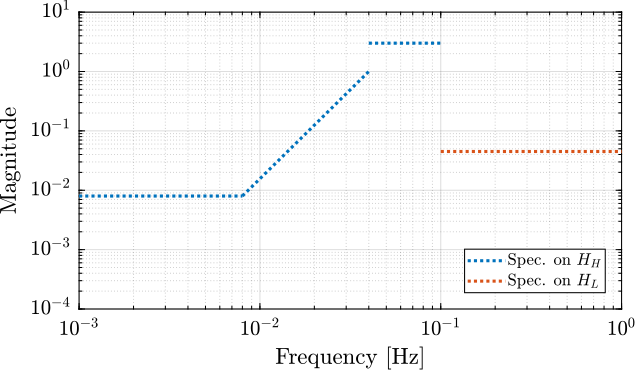
Figure 6: Specification for the LIGO complementary filters

2.2. FIR Filter

To replicated the complementary filters developed in (Hua, Adhikari, et al. 2004), the CVX Matlab toolbox (Grant and Boyd 2014) is used.

The CVX toolbox is initialized and the SeDuMi solver (Sturm 1999) is used.

%% Initialized CVX
cvx_startup;
cvx_solver sedumi;

We define the frequency vectors on which we will constrain the norm of the FIR filter.

%% Frequency vectors
w1 = 0:4.06e-4:0.008;
w2 = 0.008:4.06e-4:0.04;
w3 = 0.04:8.12e-4:0.1;
w4 = 0.1:8.12e-4:0.83;

The order \(n\) of the FIR filter is defined.

%% Filter order
n = 512;

%% Initialization of filter responses
A1 = [ones(length(w1),1),  cos(kron(w1'.*(2*pi),[1:n-1]))];
A2 = [ones(length(w2),1),  cos(kron(w2'.*(2*pi),[1:n-1]))];
A3 = [ones(length(w3),1),  cos(kron(w3'.*(2*pi),[1:n-1]))];
A4 = [ones(length(w4),1),  cos(kron(w4'.*(2*pi),[1:n-1]))];

B1 = [zeros(length(w1),1), sin(kron(w1'.*(2*pi),[1:n-1]))];
B2 = [zeros(length(w2),1), sin(kron(w2'.*(2*pi),[1:n-1]))];
B3 = [zeros(length(w3),1), sin(kron(w3'.*(2*pi),[1:n-1]))];
B4 = [zeros(length(w4),1), sin(kron(w4'.*(2*pi),[1:n-1]))];

And the convex optimization is run.

%% Convex optimization
cvx_begin

variable y(n+1,1)

% t
maximize(-y(1))

for i = 1:length(w1)
    norm([0 A1(i,:); 0 B1(i,:)]*y) <= 8e-3;
end

for  i = 1:length(w2)
    norm([0 A2(i,:); 0 B2(i,:)]*y) <= 8e-3*(2*pi*w2(i)/(0.008*2*pi))^3;
end

for i = 1:length(w3)
    norm([0 A3(i,:); 0 B3(i,:)]*y) <= 3;
end

for i = 1:length(w4)
    norm([[1 0]'- [0 A4(i,:); 0 B4(i,:)]*y]) <= y(1);
end

cvx_end

h = y(2:end);

cvx_begin
variable y(n+1,1)
% t
maximize(-y(1))
for i = 1:length(w1)
    norm([0 A1(i,:); 0 B1(i,:)]*y) <= 8e-3;
end
for  i = 1:length(w2)
    norm([0 A2(i,:); 0 B2(i,:)]*y) <= 8e-3*(2*pi*w2(i)/(0.008*2*pi))^3;
end
for i = 1:length(w3)
    norm([0 A3(i,:); 0 B3(i,:)]*y) <= 3;
end
for i = 1:length(w4)
    norm([[1 0]'- [0 A4(i,:); 0 B4(i,:)]*y]) <= y(1);
end
cvx_end

Calling SeDuMi 1.34: 4291 variables, 1586 equality constraints
   For improved efficiency, SeDuMi is solving the dual problem.
------------------------------------------------------------
SeDuMi 1.34 (beta) by AdvOL, 2005-2008 and Jos F. Sturm, 1998-2003.
Alg = 2: xz-corrector, Adaptive Step-Differentiation, theta = 0.250, beta = 0.500
eqs m = 1586, order n = 3220, dim = 4292, blocks = 1073
nnz(A) = 1100727 + 0, nnz(ADA) = 1364794, nnz(L) = 683190
 it :     b*y       gap    delta  rate   t/tP*  t/tD*   feas cg cg  prec
  0 :            4.11E+02 0.000
  1 :  -2.58E+00 1.25E+02 0.000 0.3049 0.9000 0.9000   4.87  1  1  3.0E+02
  2 :  -2.36E+00 3.90E+01 0.000 0.3118 0.9000 0.9000   1.83  1  1  6.6E+01
  3 :  -1.69E+00 1.31E+01 0.000 0.3354 0.9000 0.9000   1.76  1  1  1.5E+01
  4 :  -8.60E-01 7.10E+00 0.000 0.5424 0.9000 0.9000   2.48  1  1  4.8E+00
  5 :  -4.91E-01 5.44E+00 0.000 0.7661 0.9000 0.9000   3.12  1  1  2.5E+00
  6 :  -2.96E-01 3.88E+00 0.000 0.7140 0.9000 0.9000   2.62  1  1  1.4E+00
  7 :  -1.98E-01 2.82E+00 0.000 0.7271 0.9000 0.9000   2.14  1  1  8.5E-01
  8 :  -1.39E-01 2.00E+00 0.000 0.7092 0.9000 0.9000   1.78  1  1  5.4E-01
  9 :  -9.99E-02 1.30E+00 0.000 0.6494 0.9000 0.9000   1.51  1  1  3.3E-01
 10 :  -7.57E-02 8.03E-01 0.000 0.6175 0.9000 0.9000   1.31  1  1  2.0E-01
 11 :  -5.99E-02 4.22E-01 0.000 0.5257 0.9000 0.9000   1.17  1  1  1.0E-01
 12 :  -5.28E-02 2.45E-01 0.000 0.5808 0.9000 0.9000   1.08  1  1  5.9E-02
 13 :  -4.82E-02 1.28E-01 0.000 0.5218 0.9000 0.9000   1.05  1  1  3.1E-02
 14 :  -4.56E-02 5.65E-02 0.000 0.4417 0.9045 0.9000   1.02  1  1  1.4E-02
 15 :  -4.43E-02 2.41E-02 0.000 0.4265 0.9004 0.9000   1.01  1  1  6.0E-03
 16 :  -4.37E-02 8.90E-03 0.000 0.3690 0.9070 0.9000   1.00  1  1  2.3E-03
 17 :  -4.35E-02 3.24E-03 0.000 0.3641 0.9164 0.9000   1.00  1  1  9.5E-04
 18 :  -4.34E-02 1.55E-03 0.000 0.4788 0.9086 0.9000   1.00  1  1  4.7E-04
 19 :  -4.34E-02 8.77E-04 0.000 0.5653 0.9169 0.9000   1.00  1  1  2.8E-04
 20 :  -4.34E-02 5.05E-04 0.000 0.5754 0.9034 0.9000   1.00  1  1  1.6E-04
 21 :  -4.34E-02 2.94E-04 0.000 0.5829 0.9136 0.9000   1.00  1  1  9.9E-05
 22 :  -4.34E-02 1.63E-04 0.015 0.5548 0.9000 0.0000   1.00  1  1  6.6E-05
 23 :  -4.33E-02 9.42E-05 0.000 0.5774 0.9053 0.9000   1.00  1  1  3.9E-05
 24 :  -4.33E-02 6.27E-05 0.000 0.6658 0.9148 0.9000   1.00  1  1  2.6E-05
 25 :  -4.33E-02 3.75E-05 0.000 0.5972 0.9187 0.9000   1.00  1  1  1.6E-05
 26 :  -4.33E-02 1.89E-05 0.000 0.5041 0.9117 0.9000   1.00  1  1  8.6E-06
 27 :  -4.33E-02 9.72E-06 0.000 0.5149 0.9050 0.9000   1.00  1  1  4.5E-06
 28 :  -4.33E-02 2.94E-06 0.000 0.3021 0.9194 0.9000   1.00  1  1  1.5E-06
 29 :  -4.33E-02 9.73E-07 0.000 0.3312 0.9189 0.9000   1.00  2  2  5.3E-07
 30 :  -4.33E-02 2.82E-07 0.000 0.2895 0.9063 0.9000   1.00  2  2  1.6E-07
 31 :  -4.33E-02 8.05E-08 0.000 0.2859 0.9049 0.9000   1.00  2  2  4.7E-08
 32 :  -4.33E-02 1.43E-08 0.000 0.1772 0.9059 0.9000   1.00  2  2  8.8E-09

iter seconds digits       c*x               b*y
 32     49.4   6.8 -4.3334083581e-02 -4.3334090214e-02
|Ax-b| =   3.7e-09, [Ay-c]_+ =   1.1E-10, |x|=  1.0e+00, |y|=  2.6e+00

Detailed timing (sec)
   Pre          IPM          Post
3.902E+00    4.576E+01    1.035E-02
Max-norms: ||b||=1, ||c|| = 3,
Cholesky |add|=0, |skip| = 0, ||L.L|| = 4.26267.
------------------------------------------------------------
Status: Solved
Optimal value (cvx_optval): -0.0433341
h = y(2:end);

Finally, the filter response is computed over the frequency vector defined and the result is shown on figure 7 which is very close to the filters obtain in (Hua, Adhikari, et al. 2004).

%% Combine the frequency vectors to form the obtained filter
w = [w1 w2 w3 w4];
H = [exp(-j*kron(w'.*2*pi,[0:n-1]))]*h;

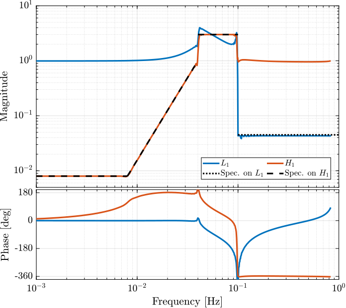
Figure 7: FIR Complementary filters obtain after convex optimization

2.3. Weighting function design

The weightings function that will be used for the \(\mathcal{H}_\infty\) synthesis of the complementary filters are now designed.

These weights will determine the order of the obtained filters.

Here are the requirements on the filters:

reasonable order
to be as close as possible to the specified upper bounds
stable and minimum phase

The weighting function for the High Pass filter is defined as follows:

%% Design of the weight for the high pass filter
w1 = 2*pi*0.008; x1 = 0.35;
w2 = 2*pi*0.04;  x2 = 0.5;
w3 = 2*pi*0.05;  x3 = 0.5;

% Slope of +3 from w1
wH = 0.008*(s^2/w1^2 + 2*x1/w1*s + 1)*(s/w1 + 1);
% Little bump from w2 to w3
wH = wH*(s^2/w2^2 + 2*x2/w2*s + 1)/(s^2/w3^2 + 2*x3/w3*s + 1);
% No Slope at high frequencies
wH = wH/(s^2/w3^2 + 2*x3/w3*s + 1)/(s/w3 + 1);
% Little bump between w2 and w3
w0 = 2*pi*0.045; xi = 0.1; A = 2; n = 1;
wH = wH*((s^2 + 2*w0*xi*A^(1/n)*s + w0^2)/(s^2 + 2*w0*xi*s + w0^2))^n;

wH = 1/wH;
wH = minreal(ss(wH));

And the weighting function for the Low pass filter is taken as a Chebyshev Type I filter.

%% Design of the weight for the low pass filter
n = 20; % Filter order
Rp = 1; % Peak to peak passband ripple
Wp = 2*pi*0.102; % Edge frequency

% Chebyshev Type I filter design
[b,a] = cheby1(n, Rp, Wp, 'high', 's');
wL = 0.04*tf(a, b);

wL = 1/wL;
wL = minreal(ss(wL));

The inverse magnitude of the weighting functions are shown in Figure 8.

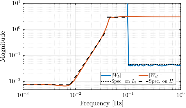
Figure 8: Weights for the \(\mathcal{H}_\infty\) synthesis

2.4. Synthesis of the complementary filters

The generalized plant of figure 1 is defined.

%% Generalized plant for the H-infinity Synthesis
P = [0   wL;
     wH -wH;
     1   0];

And the standard \(\mathcal{H}_\infty\) synthesis using the hinfsyn command is performed.

%% Standard H-Infinity synthesis
[Hl, ~, gamma, ~] = hinfsyn(P, 1, 1,'TOLGAM', 0.001, 'METHOD', 'ric', 'DISPLAY', 'on');

[Hl, ~, gamma, ~] = hinfsyn(P, 1, 1,'TOLGAM', 0.001, 'METHOD', 'ric', 'DISPLAY', 'on');
Resetting value of Gamma min based on D_11, D_12, D_21 terms

Test bounds:      0.3276 <  gamma  <=      1.8063

  gamma    hamx_eig  xinf_eig  hamy_eig   yinf_eig   nrho_xy   p/f
    1.806   1.4e-02 -1.7e-16   3.6e-03   -4.8e-12    0.0000    p
    1.067   1.3e-02 -4.2e-14   3.6e-03   -1.9e-12    0.0000    p
    0.697   1.3e-02 -3.0e-01#  3.6e-03   -3.5e-11    0.0000    f
    0.882   1.3e-02 -9.5e-01#  3.6e-03   -1.2e-34    0.0000    f
    0.975   1.3e-02 -2.7e+00#  3.6e-03   -1.6e-12    0.0000    f
    1.021   1.3e-02 -8.7e+00#  3.6e-03   -4.5e-16    0.0000    f
    1.044   1.3e-02 -6.5e-14   3.6e-03   -3.0e-15    0.0000    p
    1.032   1.3e-02 -1.8e+01#  3.6e-03    0.0e+00    0.0000    f
    1.038   1.3e-02 -3.8e+01#  3.6e-03    0.0e+00    0.0000    f
    1.041   1.3e-02 -8.3e+01#  3.6e-03   -2.9e-33    0.0000    f
    1.042   1.3e-02 -1.9e+02#  3.6e-03   -3.4e-11    0.0000    f
    1.043   1.3e-02 -5.3e+02#  3.6e-03   -7.5e-13    0.0000    f

 Gamma value achieved:     1.0439

The obtained \(\mathcal{H}_\infty\) norm is found to be close than one meaning the synthesis is successful.

The high pass filter \(H_H(s)\) is defined to be the complementary of the synthesized low pass filter \(H_L(s)\):

\begin{equation} H_H(s) = 1 - H_L(s) \end{equation}

%% High pass filter as the complementary of the low pass filter
Hh = 1 - Hl;

The size of the filters is shown to be equal to the sum of the weighting functions orders.

size(Hh), size(Hl)
State-space model with 1 outputs, 1 inputs, and 27 states.
State-space model with 1 outputs, 1 inputs, and 27 states.

The magnitude of the obtained filters as well as the requirements are shown in Figure 9.

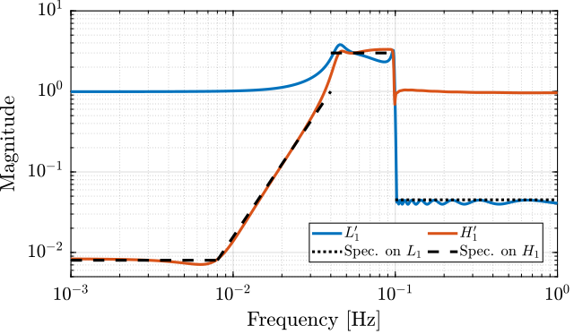
Figure 9: Obtained complementary filters using the \(\mathcal{H}_\infty\) synthesis

2.5. Comparison of the FIR filters and synthesized filters

Let’s now compare the FIR filters designed in (Hua, Adhikari, et al. 2004) with the with complementary filters obtained with the \(\mathcal{H}_\infty\) synthesis.

This is done in Figure 10, and both set of filters are found to be very close to each other.

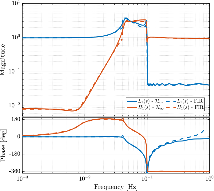
Figure 10: Comparison between the FIR filters developped for LIGO and the \(\mathcal{H}_\infty\) complementary filters

3. “Closed-Loop” complementary filters

In this section, the classical feedback architecture shown in Figure 11 is used for the design of complementary filters.

Figure 11: “Closed-Loop” complementary filters

The complete Matlab script for this part is given in Section 5.3.

3.1. Weighting Function design

Weighting functions using the generateWF Matlab function are designed to specify the upper bounds of the complementary filters to be designed. These weighting functions are the same as the ones used in Section 1.3.

%% Design of the Weighting Functions
W1 = generateWF('n', 3, 'w0', 2*pi*10, 'G0', 1000, 'Ginf', 1/10, 'Gc', 0.45);
W2 = generateWF('n', 2, 'w0', 2*pi*10, 'G0', 1/10, 'Ginf', 1000, 'Gc', 0.45);

3.2. Generalized plant

The generalized plant of Figure 12 is defined below:

%% Generalized plant for "closed-loop" complementary filter synthesis
P = [ W1 0   1;
     -W1 W2 -1];

Figure 12: Generalized plant used for the \(\mathcal{H}_\infty\) synthesis of “closed-loop” complementary filters

3.3. Synthesis of the closed-loop complementary filters

And the standard \(\mathcal{H}_\infty\) synthesis is performed.

%% Standard H-Infinity Synthesis
[L, ~, gamma, ~] = hinfsyn(P, 1, 1,'TOLGAM', 0.001, 'METHOD', 'ric', 'DISPLAY', 'on');

  Test bounds:  0.3191 <=  gamma  <=  1.669

    gamma        X>=0        Y>=0       rho(XY)<1    p/f
  7.299e-01    -1.5e-19    -2.4e+01 #   1.555e-18     f
  1.104e+00     0.0e+00     1.6e-07     2.037e-19     p
  8.976e-01    -3.2e-16    -1.4e+02 #   5.561e-16     f
  9.954e-01     0.0e+00     1.6e-07     1.041e-15     p
  9.452e-01    -1.1e-15    -3.8e+02 #   4.267e-15     f
  9.700e-01    -6.5e-16    -1.6e+03 #   9.876e-15     f
  9.826e-01     0.0e+00     1.6e-07     8.775e-39     p
  9.763e-01    -5.0e-16    -6.2e+03 #   3.519e-14     f
  9.795e-01     0.0e+00     1.6e-07     6.971e-20     p
  9.779e-01    -1.9e-31    -2.2e+04 #   5.600e-18     f
  9.787e-01     0.0e+00     1.6e-07     5.546e-19     p
  Limiting gains...
  9.789e-01     0.0e+00     1.6e-07     1.084e-13     p
  9.789e-01     0.0e+00     9.7e-07     1.137e-13     p

  Best performance (actual): 0.9789

3.4. Synthesized filters

The obtained filter \(L(s)\) can then be included in the feedback architecture shown in Figure 13.

The closed-loop transfer functions from \(\hat{x}_1\) to \(\hat{x}\) and from \(\hat{x}_2\) to \(\hat{x}\) corresponding respectively to the sensitivity and complementary sensitivity transfer functions are defined below:

%% Complementary filters
H1 = inv(1 + L);
H2 = 1 - H1;

zpk(H1) =
            (s+3.842)^3 (s+153.6) (s+1.289e05)
  -------------------------------------------------------
  (s+1.29e05) (s^2 + 102.1s + 2733) (s^2 + 69.45s + 3272)

zpk(H2) =
         125.61 (s+3358)^2 (s^2 + 46.61s + 813.8)
  -------------------------------------------------------
  (s+1.29e05) (s^2 + 102.1s + 2733) (s^2 + 69.45s + 3272)

The bode plots of the synthesized complementary filters are compared with the upper bounds in Figure 13.

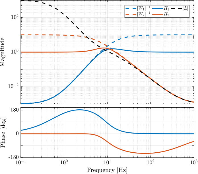
Figure 13: Bode plot of the obtained complementary filters

4. Synthesis of three complementary filters

In this section, the proposed synthesis method of complementary filters is generalized for the synthesis of a set of three complementary filters.

The complete Matlab script for this part is given in Section 5.4.

4.1. Synthesis Architecture

The synthesis objective is to shape three filters that are complementary. This corresponds to the conditions \eqref{eq:obj_three_cf} where \(W_1(s)\), \(W_2(s)\) and \(W_3(s)\) are weighting functions used to specify the maximum wanted magnitude of the three complementary filters.

\begin{equation} \begin{aligned} & |H_1(j\omega)| < \frac{1}{|W_1(j\omega)|}, \quad \forall\omega \\ & |H_2(j\omega)| < \frac{1}{|W_2(j\omega)|}, \quad \forall\omega \\ & |H_3(j\omega)| < \frac{1}{|W_3(j\omega)|}, \quad \forall\omega \\ & H_1(s) + H_2(s) + H_3(s) = 1 \end{aligned} \label{eq:obj_three_cf} \end{equation}

This synthesis can be done by performing the standard \(\mathcal{H}_\infty\) synthesis with on the generalized plant in Figure 14.

Figure 14: Generalized architecture for generating 3 complementary filters

After synthesis, filter \(H_2(s)\) and \(H_3(s)\) are obtained as shown in Figure 14. The last filter \(H_1(s)\) is defined as the complementary of the two others as in \eqref{eq:H1_complementary_of_H2_H3}.

\begin{equation} H_1(s) = 1 - H_2(s) - H_3(s) \label{eq:H1_complementary_of_H2_H3} \end{equation}

4.2. Weights

The three weighting functions are defined as shown below.

%% Design of the Weighting Functions
W1 = generateWF('n', 2, 'w0', 2*pi*1, 'G0', 1/10, 'Ginf', 1000, 'Gc', 0.5);
W2 = 0.22*(1 + s/2/pi/1)^2/(sqrt(1e-4) + s/2/pi/1)^2*(1 + s/2/pi/10)^2/(1 + s/2/pi/1000)^2;
W3 = generateWF('n', 3, 'w0', 2*pi*10, 'G0', 1000, 'Ginf', 1/10, 'Gc', 0.5);

Their inverse magnitudes are displayed in Figure 15.

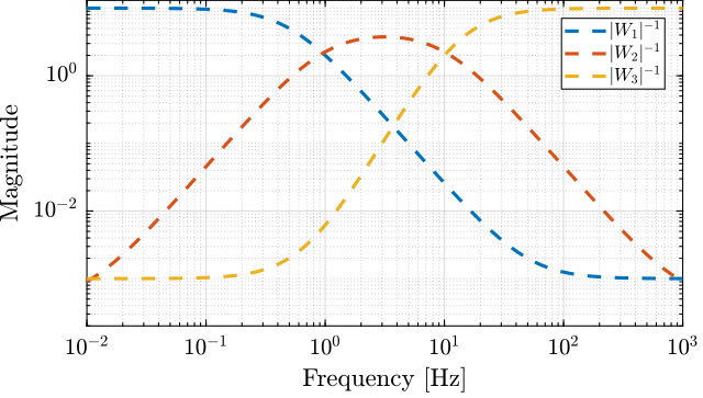
Figure 15: Three weighting functions used for the \(\mathcal{H}_\infty\) synthesis of the complementary filters

4.3. H-Infinity Synthesis

The generalized plant in Figure 14 containing the weighting functions is defined below.

%% Generalized plant for the synthesis of 3 complementary filters
P = [W1 -W1 -W1;
     0   W2  0 ;
     0   0   W3;
     1   0   0];

And the standard \(\mathcal{H}_\infty\) synthesis using the hinfsyn command is performed.

%% Standard H-Infinity Synthesis
[H, ~, gamma, ~] = hinfsyn(P, 1, 2,'TOLGAM', 0.001, 'METHOD', 'ric', 'DISPLAY', 'on');

Resetting value of Gamma min based on D_11, D_12, D_21 terms

Test bounds:      0.1000 <  gamma  <=   1050.0000

  gamma    hamx_eig  xinf_eig  hamy_eig   yinf_eig   nrho_xy   p/f
1.050e+03   3.2e+00   4.5e-13   6.3e-02   -1.2e-11    0.0000    p
  525.050   3.2e+00   1.3e-13   6.3e-02    0.0e+00    0.0000    p
  262.575   3.2e+00   2.1e-12   6.3e-02   -1.5e-13    0.0000    p
  131.337   3.2e+00   1.1e-12   6.3e-02   -7.2e-29    0.0000    p
   65.719   3.2e+00   2.0e-12   6.3e-02    0.0e+00    0.0000    p
   32.909   3.2e+00   7.4e-13   6.3e-02   -5.9e-13    0.0000    p
   16.505   3.2e+00   1.4e-12   6.3e-02    0.0e+00    0.0000    p
    8.302   3.2e+00   1.6e-12   6.3e-02    0.0e+00    0.0000    p
    4.201   3.2e+00   1.6e-12   6.3e-02    0.0e+00    0.0000    p
    2.151   3.2e+00   1.6e-12   6.3e-02    0.0e+00    0.0000    p
    1.125   3.2e+00   2.8e-12   6.3e-02    0.0e+00    0.0000    p
    0.613   3.0e+00 -2.5e+03#  6.3e-02    0.0e+00    0.0000    f
    0.869   3.1e+00 -2.9e+01#  6.3e-02    0.0e+00    0.0000    f
    0.997   3.2e+00   1.9e-12   6.3e-02    0.0e+00    0.0000    p
    0.933   3.1e+00 -6.9e+02#  6.3e-02    0.0e+00    0.0000    f
    0.965   3.1e+00 -3.0e+03#  6.3e-02    0.0e+00    0.0000    f
    0.981   3.1e+00 -8.6e+03#  6.3e-02    0.0e+00    0.0000    f
    0.989   3.2e+00 -2.7e+04#  6.3e-02    0.0e+00    0.0000    f
    0.993   3.2e+00 -5.7e+05#  6.3e-02    0.0e+00    0.0000    f
    0.995   3.2e+00   2.2e-12   6.3e-02    0.0e+00    0.0000    p
    0.994   3.2e+00   1.6e-12   6.3e-02    0.0e+00    0.0000    p
    0.994   3.2e+00   1.0e-12   6.3e-02    0.0e+00    0.0000    p

 Gamma value achieved:     0.9936

The two synthesized filters \(H_2(s)\) and \(H_3(s)\) are defined below: And the third filter \(H_1(s)\) is defined using \eqref{eq:H1_complementary_of_H2_H3}.

%% H1 is defined as the complementary filter of H2 and H3
H1 = 1 - H2 - H3;

The bode plots of the three obtained complementary filters are shown in Figure 16.

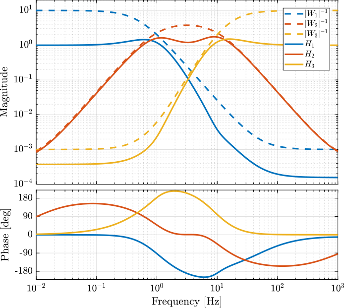
Figure 16: The three complementary filters obtained after \(\mathcal{H}_\infty\) synthesis

5. Matlab Scripts

5.1. `1_synthesis_complementary_filters.m`

This scripts corresponds to section 3 of (Dehaeze, Vermat, and Collette 2004).

  1: %% Clear Workspace and Close figures
  2: clear; close all; clc;
  3: 
  4: %% Intialize Laplace variable
  5: s = zpk('s');
  6: 
  7: %% Initialize Frequency Vector
  8: freqs = logspace(-1, 3, 1000);
  9: 
 10: %% Add functions to path
 11: addpath('./src');
 12: 
 13: %% Weighting Function Design
 14: % Parameters
 15: n = 3; w0 = 2*pi*10; G0 = 1e-3; G1 = 1e1; Gc = 2;
 16: 
 17: % Formulas
 18: W = (((1/w0)*sqrt((1-(G0/Gc)^(2/n))/(1-(Gc/G1)^(2/n)))*s + (G0/Gc)^(1/n))/((1/G1)^(1/n)*(1/w0)*sqrt((1-(G0/Gc)^(2/n))/(1-(Gc/G1)^(2/n)))*s + (1/Gc)^(1/n)))^n;
 19: 
 20: %% Magnitude of the weighting function with parameters
 21: figure;
 22: hold on;
 23: plot(freqs, abs(squeeze(freqresp(W, freqs, 'Hz'))), 'k-');
 24: 
 25: plot([1e-3 1e0], [G0 G0], 'k--', 'LineWidth', 1)
 26: text(1e0, G0, '$\quad G_0$')
 27: 
 28: plot([1e1 1e3], [G1 G1], 'k--', 'LineWidth', 1)
 29: text(1e1,G1,'$G_{\infty}\quad$','HorizontalAlignment', 'right')
 30: 
 31: plot([w0/2/pi w0/2/pi], [1 2*Gc], 'k--', 'LineWidth', 1)
 32: text(w0/2/pi,1,'$\omega_c$','VerticalAlignment', 'top', 'HorizontalAlignment', 'center')
 33: 
 34: plot([w0/2/pi/2  2*w0/2/pi], [Gc Gc], 'k--', 'LineWidth', 1)
 35: text(w0/2/pi/2, Gc, '$G_c \quad$','HorizontalAlignment', 'right')
 36: 
 37: text(w0/5/pi/2, abs(evalfr(W, j*w0/5)), 'Slope: $n \quad$', 'HorizontalAlignment', 'right')
 38: 
 39: text(w0/2/pi, abs(evalfr(W, j*w0)), '$\bullet$', 'HorizontalAlignment', 'center')
 40: set(gca, 'XScale', 'log'); set(gca, 'YScale', 'log');
 41: xlabel('Frequency [Hz]'); ylabel('Magnitude');
 42: hold off;
 43: xlim([freqs(1), freqs(end)]);
 44: ylim([5e-4, 20]);
 45: yticks([1e-4, 1e-3, 1e-2, 1e-1, 1, 1e1]);
 46: 
 47: %% Design of the Weighting Functions
 48: W1 = generateWF('n', 3, 'w0', 2*pi*10, 'G0', 1000, 'G1', 1/10, 'Gc', 0.45);
 49: W2 = generateWF('n', 2, 'w0', 2*pi*10, 'G0', 1/10, 'G1', 1000, 'Gc', 0.45);
 50: 
 51: %% Plot of the Weighting function magnitude
 52: figure;
 53: tiledlayout(1, 1, 'TileSpacing', 'None', 'Padding', 'None');
 54: ax1 = nexttile();
 55: hold on;
 56: set(gca,'ColorOrderIndex',1)
 57: plot(freqs, 1./abs(squeeze(freqresp(W1, freqs, 'Hz'))), '--', 'DisplayName', '$|W_1|^{-1}$');
 58: set(gca,'ColorOrderIndex',2)
 59: plot(freqs, 1./abs(squeeze(freqresp(W2, freqs, 'Hz'))), '--', 'DisplayName', '$|W_2|^{-1}$');
 60: set(gca, 'XScale', 'log'); set(gca, 'YScale', 'log');
 61: xlabel('Frequency [Hz]', 'FontSize', 10); ylabel('Magnitude', 'FontSize', 10);
 62: hold off;
 63: xlim([freqs(1), freqs(end)]);
 64: xticks([0.1, 1, 10, 100, 1000]);
 65: ylim([8e-4, 20]);
 66: yticks([1e-3, 1e-2, 1e-1, 1, 1e1]);
 67: yticklabels({'', '$10^{-2}$', '', '$10^0$', ''});
 68: ax1.FontSize = 9;
 69: leg = legend('location', 'south', 'FontSize', 8);
 70: leg.ItemTokenSize(1) = 18;
 71: 
 72: %% Generalized Plant
 73: P = [W1 -W1;
 74:      0   W2;
 75:      1   0];
 76: 
 77: %% H-Infinity Synthesis
 78: [H2, ~, gamma, ~] = hinfsyn(P, 1, 1,'TOLGAM', 0.001, 'METHOD', 'ric', 'DISPLAY', 'on');
 79: 
 80: %% Define H1 to be the complementary of H2
 81: H1 = 1 - H2;
 82: 
 83: %% Bode plot of the complementary filters
 84: figure;
 85: tiledlayout(3, 1, 'TileSpacing', 'None', 'Padding', 'None');
 86: 
 87: % Magnitude
 88: ax1 = nexttile([2, 1]);
 89: hold on;
 90: set(gca,'ColorOrderIndex',1)
 91: plot(freqs, 1./abs(squeeze(freqresp(W1, freqs, 'Hz'))), '--', 'DisplayName', '$|W_1|^{-1}$');
 92: set(gca,'ColorOrderIndex',2)
 93: plot(freqs, 1./abs(squeeze(freqresp(W2, freqs, 'Hz'))), '--', 'DisplayName', '$|W_2|^{-1}$');
 94: 
 95: set(gca,'ColorOrderIndex',1)
 96: plot(freqs, abs(squeeze(freqresp(H1, freqs, 'Hz'))), '-', 'DisplayName', '$H_1$');
 97: set(gca,'ColorOrderIndex',2)
 98: plot(freqs, abs(squeeze(freqresp(H2, freqs, 'Hz'))), '-', 'DisplayName', '$H_2$');
 99: hold off;
100: set(gca, 'XScale', 'log'); set(gca, 'YScale', 'log');
101: set(gca, 'XTickLabel',[]); ylabel('Magnitude');
102: ylim([8e-4, 20]);
103: yticks([1e-3, 1e-2, 1e-1, 1, 1e1]);
104: yticklabels({'', '$10^{-2}$', '', '$10^0$', ''})
105: leg = legend('location', 'south', 'FontSize', 8, 'NumColumns', 2);
106: leg.ItemTokenSize(1) = 18;
107: 
108: % Phase
109: ax2 = nexttile;
110: hold on;
111: set(gca,'ColorOrderIndex',1)
112: plot(freqs, 180/pi*phase(squeeze(freqresp(H1, freqs, 'Hz'))), '-');
113: set(gca,'ColorOrderIndex',2)
114: plot(freqs, 180/pi*phase(squeeze(freqresp(H2, freqs, 'Hz'))), '-');
115: hold off;
116: set(gca, 'XScale', 'log');
117: xlabel('Frequency [Hz]'); ylabel('Phase [deg]');
118: yticks([-180:90:180]);
119: ylim([-180, 200])
120: yticklabels({'-180', '', '0', '', '180'})
121: 
122: linkaxes([ax1,ax2],'x');
123: xlim([freqs(1), freqs(end)]);

5.2. `2_ligo_complementary_filters.m`

This scripts corresponds to section 4 of (Dehaeze, Vermat, and Collette 2004).

  1: %% Clear Workspace and Close figures
  2: clear; close all; clc;
  3: 
  4: %% Intialize Laplace variable
  5: s = zpk('s');
  6: 
  7: %% Initialize Frequency Vector
  8: freqs = logspace(-3, 0, 1000);
  9: 
 10: %% Add functions to path
 11: addpath('./src');
 12: 
 13: %% Upper bounds for the complementary filters
 14: figure;
 15: hold on;
 16: set(gca,'ColorOrderIndex',1)
 17: plot([0.0001, 0.008], [8e-3, 8e-3], ':', 'DisplayName', 'Spec. on $H_H$');
 18: set(gca,'ColorOrderIndex',1)
 19: plot([0.008 0.04], [8e-3, 1], ':', 'HandleVisibility', 'off');
 20: set(gca,'ColorOrderIndex',1)
 21: plot([0.04 0.1], [3, 3], ':', 'HandleVisibility', 'off');
 22: set(gca,'ColorOrderIndex',2)
 23: plot([0.1, 10], [0.045, 0.045], ':', 'DisplayName', 'Spec. on $H_L$');
 24: set(gca, 'XScale', 'log'); set(gca, 'YScale', 'log');
 25: xlabel('Frequency [Hz]'); ylabel('Magnitude');
 26: hold off;
 27: xlim([freqs(1), freqs(end)]);
 28: ylim([1e-4, 10]);
 29: leg = legend('location', 'southeast', 'FontSize', 8);
 30: leg.ItemTokenSize(1) = 18;
 31: 
 32: %% Initialized CVX
 33: cvx_startup;
 34: cvx_solver sedumi;
 35: 
 36: %% Frequency vectors
 37: w1 = 0:4.06e-4:0.008;
 38: w2 = 0.008:4.06e-4:0.04;
 39: w3 = 0.04:8.12e-4:0.1;
 40: w4 = 0.1:8.12e-4:0.83;
 41: 
 42: %% Filter order
 43: n = 512;
 44: 
 45: %% Initialization of filter responses
 46: A1 = [ones(length(w1),1),  cos(kron(w1'.*(2*pi),[1:n-1]))];
 47: A2 = [ones(length(w2),1),  cos(kron(w2'.*(2*pi),[1:n-1]))];
 48: A3 = [ones(length(w3),1),  cos(kron(w3'.*(2*pi),[1:n-1]))];
 49: A4 = [ones(length(w4),1),  cos(kron(w4'.*(2*pi),[1:n-1]))];
 50: 
 51: B1 = [zeros(length(w1),1), sin(kron(w1'.*(2*pi),[1:n-1]))];
 52: B2 = [zeros(length(w2),1), sin(kron(w2'.*(2*pi),[1:n-1]))];
 53: B3 = [zeros(length(w3),1), sin(kron(w3'.*(2*pi),[1:n-1]))];
 54: B4 = [zeros(length(w4),1), sin(kron(w4'.*(2*pi),[1:n-1]))];
 55: 
 56: %% Convex optimization
 57: cvx_begin
 58: 
 59: variable y(n+1,1)
 60: 
 61: % t
 62: maximize(-y(1))
 63: 
 64: for i = 1:length(w1)
 65:     norm([0 A1(i,:); 0 B1(i,:)]*y) <= 8e-3;
 66: end
 67: 
 68: for  i = 1:length(w2)
 69:     norm([0 A2(i,:); 0 B2(i,:)]*y) <= 8e-3*(2*pi*w2(i)/(0.008*2*pi))^3;
 70: end
 71: 
 72: for i = 1:length(w3)
 73:     norm([0 A3(i,:); 0 B3(i,:)]*y) <= 3;
 74: end
 75: 
 76: for i = 1:length(w4)
 77:     norm([[1 0]'- [0 A4(i,:); 0 B4(i,:)]*y]) <= y(1);
 78: end
 79: 
 80: cvx_end
 81: 
 82: h = y(2:end);
 83: 
 84: %% Combine the frequency vectors to form the obtained filter
 85: w = [w1 w2 w3 w4];
 86: H = [exp(-j*kron(w'.*2*pi,[0:n-1]))]*h;
 87: 
 88: %% Bode plot of the obtained complementary filters
 89: figure;
 90: tiledlayout(3, 1, 'TileSpacing', 'None', 'Padding', 'None');
 91: 
 92: % Magnitude
 93: ax1 = nexttile([2, 1]);
 94: hold on;
 95: set(gca,'ColorOrderIndex',1)
 96: plot(w, abs(1-H), '-', 'DisplayName', '$L_1$');
 97: plot([0.1, 10], [0.045, 0.045], 'k:', 'DisplayName', 'Spec. on $L_1$');
 98: 
 99: set(gca,'ColorOrderIndex',2)
100: plot(w, abs(H), '-', 'DisplayName', '$H_1$');
101: plot([0.0001, 0.008], [8e-3, 8e-3], 'k--', 'DisplayName', 'Spec. on $H_1$');
102: plot([0.008 0.04], [8e-3, 1],       'k--', 'HandleVisibility', 'off');
103: plot([0.04 0.1], [3, 3],            'k--', 'HandleVisibility', 'off');
104: 
105: set(gca, 'XScale', 'log'); set(gca, 'YScale', 'log');
106: set(gca, 'XTickLabel',[]); ylabel('Magnitude');
107: hold off;
108: ylim([5e-3, 10]);
109: leg = legend('location', 'southeast', 'FontSize', 8, 'NumColumns', 2);
110: leg.ItemTokenSize(1) = 16;
111: 
112: % Phase
113: ax2 = nexttile;
114: hold on;
115: plot(w, 180/pi*unwrap(angle(1-H)), '-');
116: plot(w, 180/pi*unwrap(angle(H)), '-');
117: hold off;
118: xlabel('Frequency [Hz]'); ylabel('Phase [deg]');
119: set(gca, 'XScale', 'log');
120: yticks([-360:180:180]); ylim([-380, 200]);
121: 
122: linkaxes([ax1,ax2],'x');
123: xlim([1e-3, 1]);
124: 
125: %% Design of the weight for the high pass filter
126: w1 = 2*pi*0.008; x1 = 0.35;
127: w2 = 2*pi*0.04;  x2 = 0.5;
128: w3 = 2*pi*0.05;  x3 = 0.5;
129: 
130: % Slope of +3 from w1
131: wH = 0.008*(s^2/w1^2 + 2*x1/w1*s + 1)*(s/w1 + 1);
132: % Little bump from w2 to w3
133: wH = wH*(s^2/w2^2 + 2*x2/w2*s + 1)/(s^2/w3^2 + 2*x3/w3*s + 1);
134: % No Slope at high frequencies
135: wH = wH/(s^2/w3^2 + 2*x3/w3*s + 1)/(s/w3 + 1);
136: % Little bump between w2 and w3
137: w0 = 2*pi*0.045; xi = 0.1; A = 2; n = 1;
138: wH = wH*((s^2 + 2*w0*xi*A^(1/n)*s + w0^2)/(s^2 + 2*w0*xi*s + w0^2))^n;
139: 
140: wH = 1/wH;
141: wH = minreal(ss(wH));
142: 
143: %% Design of the weight for the low pass filter
144: n = 20; % Filter order
145: Rp = 1; % Peak to peak passband ripple
146: Wp = 2*pi*0.102; % Edge frequency
147: 
148: % Chebyshev Type I filter design
149: [b,a] = cheby1(n, Rp, Wp, 'high', 's');
150: wL = 0.04*tf(a, b);
151: 
152: wL = 1/wL;
153: wL = minreal(ss(wL));
154: 
155: %% Magnitude of the designed Weights and initial specifications
156: figure;
157: hold on;
158: set(gca,'ColorOrderIndex',1);
159: plot(freqs, abs(squeeze(freqresp(inv(wL), freqs, 'Hz'))), '-', 'DisplayName', '$|W_L|^{-1}$');
160: plot([0.1, 10], [0.045, 0.045],     'k:',  'DisplayName', 'Spec. on $L_1$');
161: 
162: set(gca,'ColorOrderIndex',2);
163: plot(freqs, abs(squeeze(freqresp(inv(wH), freqs, 'Hz'))), '-', 'DisplayName', '$|W_H|^{-1}$');
164: plot([0.0001, 0.008], [8e-3, 8e-3], 'k--', 'DisplayName', 'Spec. on $H_1$');
165: plot([0.008 0.04], [8e-3, 1],       'k--', 'HandleVisibility', 'off');
166: plot([0.04 0.1], [3, 3],            'k--', 'HandleVisibility', 'off');
167: 
168: set(gca, 'XScale', 'log'); set(gca, 'YScale', 'log');
169: xlabel('Frequency [Hz]'); ylabel('Magnitude');
170: hold off;
171: xlim([freqs(1), freqs(end)]);
172: ylim([5e-3, 10]);
173: leg = legend('location', 'southeast', 'FontSize', 8, 'NumColumns', 2);
174: leg.ItemTokenSize(1) = 16;
175: 
176: %% Generalized plant for the H-infinity Synthesis
177: P = [0   wL;
178:      wH -wH;
179:      1   0];
180: 
181: %% Standard H-Infinity synthesis
182: [Hl, ~, gamma, ~] = hinfsyn(P, 1, 1,'TOLGAM', 0.001, 'METHOD', 'ric', 'DISPLAY', 'on');
183: 
184: %% High pass filter as the complementary of the low pass filter
185: Hh = 1 - Hl;
186: 
187: %% Minimum realization of the filters
188: Hh = minreal(Hh);
189: Hl = minreal(Hl);
190: 
191: %% Bode plot of the obtained filters and comparison with the upper bounds
192: figure;
193: hold on;
194: set(gca,'ColorOrderIndex',1);
195: plot(freqs, abs(squeeze(freqresp(Hl, freqs, 'Hz'))), '-', 'DisplayName', '$L_1^\prime$');
196: plot([0.1, 10], [0.045, 0.045],     'k:',  'DisplayName', 'Spec. on $L_1$');
197: 
198: set(gca,'ColorOrderIndex',2);
199: plot(freqs, abs(squeeze(freqresp(Hh, freqs, 'Hz'))), '-', 'DisplayName', '$H_1^\prime$');
200: plot([0.0001, 0.008], [8e-3, 8e-3], 'k--', 'DisplayName', 'Spec. on $H_1$');
201: plot([0.008 0.04], [8e-3, 1],       'k--', 'HandleVisibility', 'off');
202: plot([0.04 0.1], [3, 3],            'k--', 'HandleVisibility', 'off');
203: 
204: set(gca, 'XScale', 'log'); set(gca, 'YScale', 'log');
205: xlabel('Frequency [Hz]'); ylabel('Magnitude');
206: hold off;
207: xlim([freqs(1), freqs(end)]);
208: ylim([5e-3, 10]);
209: leg = legend('location', 'southeast', 'FontSize', 8, 'NumColumns', 2);
210: leg.ItemTokenSize(1) = 16;
211: 
212: %% Comparison of the complementary filters obtained with H-infinity and with CVX
213: figure;
214: tiledlayout(3, 1, 'TileSpacing', 'None', 'Padding', 'None');
215: 
216: % Magnitude
217: ax1 = nexttile([2, 1]);
218: hold on;
219: set(gca,'ColorOrderIndex',1);
220: plot(freqs, abs(squeeze(freqresp(Hl, freqs, 'Hz'))), '-', ...
221:      'DisplayName', '$L_1(s)$ - $\mathcal{H}_\infty$');
222: set(gca,'ColorOrderIndex',2);
223: plot(freqs, abs(squeeze(freqresp(Hh, freqs, 'Hz'))), '-', ...
224:      'DisplayName', '$H_1(s)$ - $\mathcal{H}_\infty$');
225: 
226: set(gca,'ColorOrderIndex',1);
227: plot(w, abs(1-H), '--', ...
228:      'DisplayName', '$L_1(s)$ - FIR');
229: set(gca,'ColorOrderIndex',2);
230: plot(w, abs(H), '--', ...
231:      'DisplayName', '$H_1(s)$ - FIR');
232: hold off;
233: set(gca, 'XScale', 'log'); set(gca, 'YScale', 'log');
234: ylabel('Magnitude');
235: set(gca, 'XTickLabel',[]);
236: ylim([5e-3, 10]);
237: leg = legend('location', 'southeast', 'FontSize', 8, 'NumColumns', 2);
238: leg.ItemTokenSize(1) = 16;
239: 
240: % Phase
241: ax2 = nexttile;
242: hold on;
243: set(gca,'ColorOrderIndex',1);
244: plot(freqs, 180/pi*unwrap(angle(squeeze(freqresp(Hl, freqs, 'Hz')))), '-');
245: set(gca,'ColorOrderIndex',2);
246: plot(freqs, 180/pi*unwrap(angle(squeeze(freqresp(Hh, freqs, 'Hz')))), '-');
247: 
248: set(gca,'ColorOrderIndex',1);
249: plot(w, 180/pi*unwrap(angle(1-H)), '--');
250: set(gca,'ColorOrderIndex',2);
251: plot(w, 180/pi*unwrap(angle(H)), '--');
252: set(gca, 'XScale', 'log');
253: xlabel('Frequency [Hz]'); ylabel('Phase [deg]');
254: hold off;
255: yticks([-360:180:180]); ylim([-380, 200]);
256: 
257: linkaxes([ax1,ax2],'x');
258: xlim([freqs(1), freqs(end)]);

5.3. `3_closed_loop_complementary_filters.m`

This scripts corresponds to section 5.1 of (Dehaeze, Vermat, and Collette 2004).

 1: %% Clear Workspace and Close figures
 2: clear; close all; clc;
 3: 
 4: %% Intialize Laplace variable
 5: s = zpk('s');
 6: 
 7: %% Initialize Frequency Vector
 8: freqs = logspace(-1, 3, 1000);
 9: 
10: %% Add functions to path
11: addpath('./src');
12: 
13: %% Design of the Weighting Functions
14: W1 = generateWF('n', 3, 'w0', 2*pi*10, 'G0', 1000, 'G1', 1/10, 'Gc', 0.45);
15: W2 = generateWF('n', 2, 'w0', 2*pi*10, 'G0', 1/10, 'G1', 1000, 'Gc', 0.45);
16: 
17: %% Generalized plant for "closed-loop" complementary filter synthesis
18: P = [ W1 0   1;
19:      -W1 W2 -1];
20: 
21: %% Standard H-Infinity Synthesis
22: [L, ~, gamma, ~] = hinfsyn(P, 1, 1,'TOLGAM', 0.001, 'METHOD', 'ric', 'DISPLAY', 'on');
23: 
24: %% Complementary filters
25: H1 = inv(1 + L);
26: H2 = 1 - H1;
27: 
28: %% Bode plot of the obtained Complementary filters with upper-bounds
29: freqs = logspace(-1, 3, 1000);
30: figure;
31: tiledlayout(3, 1, 'TileSpacing', 'None', 'Padding', 'None');
32: 
33: % Magnitude
34: ax1 = nexttile([2, 1]);
35: hold on;
36: set(gca,'ColorOrderIndex',1)
37: plot(freqs, 1./abs(squeeze(freqresp(W1, freqs, 'Hz'))), '--', 'DisplayName', '$|W_1|^{-1}$');
38: set(gca,'ColorOrderIndex',2)
39: plot(freqs, 1./abs(squeeze(freqresp(W2, freqs, 'Hz'))), '--', 'DisplayName', '$|W_2|^{-1}$');
40: 
41: set(gca,'ColorOrderIndex',1)
42: plot(freqs, abs(squeeze(freqresp(H1, freqs, 'Hz'))), '-', 'DisplayName', '$H_1$');
43: set(gca,'ColorOrderIndex',2)
44: plot(freqs, abs(squeeze(freqresp(H2, freqs, 'Hz'))), '-', 'DisplayName', '$H_2$');
45: 
46: plot(freqs, abs(squeeze(freqresp(L, freqs, 'Hz'))), 'k--', 'DisplayName', '$|L|$');
47: hold off;
48: set(gca, 'XScale', 'log'); set(gca, 'YScale', 'log');
49: set(gca, 'XTickLabel',[]); ylabel('Magnitude');
50: ylim([1e-3, 1e3]);
51: yticks([1e-3, 1e-2, 1e-1, 1, 1e1, 1e2, 1e3]);
52: yticklabels({'', '$10^{-2}$', '', '$10^0$', '', '$10^2$', ''});
53: leg = legend('location', 'northeast', 'FontSize', 8, 'NumColumns', 3);
54: leg.ItemTokenSize(1) = 18;
55: 
56: % Phase
57: ax2 = nexttile;
58: hold on;
59: set(gca,'ColorOrderIndex',1)
60: plot(freqs, 180/pi*phase(squeeze(freqresp(H1, freqs, 'Hz'))), '-');
61: set(gca,'ColorOrderIndex',2)
62: plot(freqs, 180/pi*phase(squeeze(freqresp(H2, freqs, 'Hz'))), '-');
63: hold off;
64: set(gca, 'XScale', 'log');
65: xlabel('Frequency [Hz]'); ylabel('Phase [deg]');
66: yticks([-180:90:180]);
67: ylim([-180, 200])
68: yticklabels({'-180', '', '0', '', '180'})
69: 
70: linkaxes([ax1,ax2],'x');
71: xlim([freqs(1), freqs(end)]);

5.4. `4_three_complementary_filters.m`

This scripts corresponds to section 5.2 of (Dehaeze, Vermat, and Collette 2004).

  1: %% Clear Workspace and Close figures
  2: clear; close all; clc;
  3: 
  4: %% Intialize Laplace variable
  5: s = zpk('s');
  6: 
  7: freqs = logspace(-2, 3, 1000);
  8: 
  9: addpath('./src');
 10: 
 11: % Weights
 12: % First we define the weights.
 13: 
 14: %% Design of the Weighting Functions
 15: W1 = generateWF('n', 2, 'w0', 2*pi*1, 'G0', 1/10, 'G1', 1000, 'Gc', 0.5);
 16: W2 = 0.22*(1 + s/2/pi/1)^2/(sqrt(1e-4) + s/2/pi/1)^2*(1 + s/2/pi/10)^2/(1 + s/2/pi/1000)^2;
 17: W3 = generateWF('n', 3, 'w0', 2*pi*10, 'G0', 1000, 'G1', 1/10, 'Gc', 0.5);
 18: 
 19: %% Inverse magnitude of the weighting functions
 20: figure;
 21: hold on;
 22: set(gca,'ColorOrderIndex',1)
 23: plot(freqs, 1./abs(squeeze(freqresp(W1, freqs, 'Hz'))), '--', 'DisplayName', '$|W_1|^{-1}$');
 24: set(gca,'ColorOrderIndex',2)
 25: plot(freqs, 1./abs(squeeze(freqresp(W2, freqs, 'Hz'))), '--', 'DisplayName', '$|W_2|^{-1}$');
 26: set(gca,'ColorOrderIndex',3)
 27: plot(freqs, 1./abs(squeeze(freqresp(W3, freqs, 'Hz'))), '--', 'DisplayName', '$|W_3|^{-1}$');
 28: set(gca, 'XScale', 'log'); set(gca, 'YScale', 'log');
 29: xlabel('Frequency [Hz]'); ylabel('Magnitude');
 30: hold off;
 31: xlim([freqs(1), freqs(end)]); ylim([2e-4, 1.3e1])
 32: leg = legend('location', 'northeast', 'FontSize', 8);
 33: leg.ItemTokenSize(1) = 18;
 34: 
 35: % H-Infinity Synthesis
 36: % Then we create the generalized plant =P=.
 37: 
 38: %% Generalized plant for the synthesis of 3 complementary filters
 39: P = [W1 -W1 -W1;
 40:      0   W2  0 ;
 41:      0   0   W3;
 42:      1   0   0];
 43: 
 44: 
 45: 
 46: % And we do the $\mathcal{H}_\infty$ synthesis.
 47: 
 48: %% Standard H-Infinity Synthesis
 49: [H, ~, gamma, ~] = hinfsyn(P, 1, 2,'TOLGAM', 0.001, 'METHOD', 'ric', 'DISPLAY', 'on');
 50: 
 51: % Obtained Complementary Filters
 52: % The obtained filters are:
 53: 
 54: %%
 55: H2 = tf(H(1));
 56: H3 = tf(H(2));
 57: H1 = 1 - H2 - H3;
 58: 
 59: %% Bode plot of the obtained complementary filters
 60: figure;
 61: tiledlayout(3, 1, 'TileSpacing', 'None', 'Padding', 'None');
 62: 
 63: % Magnitude
 64: ax1 = nexttile([2, 1]);
 65: hold on;
 66: set(gca,'ColorOrderIndex',1)
 67: plot(freqs, 1./abs(squeeze(freqresp(W1, freqs, 'Hz'))), '--', 'DisplayName', '$|W_1|^{-1}$');
 68: set(gca,'ColorOrderIndex',2)
 69: plot(freqs, 1./abs(squeeze(freqresp(W2, freqs, 'Hz'))), '--', 'DisplayName', '$|W_2|^{-1}$');
 70: set(gca,'ColorOrderIndex',3)
 71: plot(freqs, 1./abs(squeeze(freqresp(W3, freqs, 'Hz'))), '--', 'DisplayName', '$|W_3|^{-1}$');
 72: set(gca,'ColorOrderIndex',1)
 73: plot(freqs, abs(squeeze(freqresp(H1, freqs, 'Hz'))), '-', 'DisplayName', '$H_1$');
 74: set(gca,'ColorOrderIndex',2)
 75: plot(freqs, abs(squeeze(freqresp(H2, freqs, 'Hz'))), '-', 'DisplayName', '$H_2$');
 76: set(gca,'ColorOrderIndex',3)
 77: plot(freqs, abs(squeeze(freqresp(H3, freqs, 'Hz'))), '-', 'DisplayName', '$H_3$');
 78: set(gca, 'XScale', 'log'); set(gca, 'YScale', 'log');
 79: hold off;
 80: set(gca, 'XScale', 'log'); set(gca, 'YScale', 'log');
 81: ylabel('Magnitude');
 82: set(gca, 'XTickLabel',[]);
 83: ylim([1e-4, 20]);
 84: leg = legend('location', 'northeast', 'FontSize', 8);
 85: leg.ItemTokenSize(1) = 18;
 86: 
 87: % Phase
 88: ax2 = nexttile;
 89: hold on;
 90: set(gca,'ColorOrderIndex',1)
 91: plot(freqs, 180/pi*phase(squeeze(freqresp(H1, freqs, 'Hz'))));
 92: set(gca,'ColorOrderIndex',2)
 93: plot(freqs, 180/pi*phase(squeeze(freqresp(H2, freqs, 'Hz'))));
 94: set(gca,'ColorOrderIndex',3)
 95: plot(freqs, 180/pi*phase(squeeze(freqresp(H3, freqs, 'Hz'))));
 96: hold off;
 97: xlabel('Frequency [Hz]'); ylabel('Phase [deg]');
 98: set(gca, 'XScale', 'log');
 99: yticks([-180:90:180]); ylim([-220, 220]);
100: 
101: linkaxes([ax1,ax2],'x');
102: xlim([freqs(1), freqs(end)]);

5.5. `generateWF`: Generate Weighting Functions

This function is used to easily generate weighting functions from classical requirements.

function [W] = generateWF(args)
% createWeight -
%
% Syntax: [W] = generateWeight(args)
%
% Inputs:
%    - n  - Weight Order (integer)
%    - G0 - Low frequency Gain
%    - G1 - High frequency Gain
%    - Gc - Gain of the weight at frequency w0
%    - w0 - Frequency at which |W(j w0)| = Gc [rad/s]
%
% Outputs:
%    - W - Generated Weighting Function

%% Argument validation
arguments
    args.n    (1,1) double {mustBeInteger, mustBePositive} = 1
    args.G0   (1,1) double {mustBeNumeric, mustBePositive} = 0.1
    args.Ginf (1,1) double {mustBeNumeric, mustBePositive} = 10
    args.Gc   (1,1) double {mustBeNumeric, mustBePositive} = 1
    args.w0   (1,1) double {mustBeNumeric, mustBePositive} = 1
end

% Verification of correct relation between G0, Gc and Ginf
mustBeBetween(args.G0, args.Gc, args.Ginf);

%% Initialize the Laplace variable
s = zpk('s');

%% Create the weighting function according to formula
W = (((1/args.w0)*sqrt((1-(args.G0/args.Gc)^(2/args.n))/(1-(args.Gc/args.Ginf)^(2/args.n)))*s + ...
      (args.G0/args.Gc)^(1/args.n))/...
     ((1/args.Ginf)^(1/args.n)*(1/args.w0)*sqrt((1-(args.G0/args.Gc)^(2/args.n))/(1-(args.Gc/args.Ginf)^(2/args.n)))*s + ...
      (1/args.Gc)^(1/args.n)))^args.n;

%% Custom validation function
function mustBeBetween(a,b,c)
    if ~((a > b && b > c) || (c > b && b > a))
        eid = 'createWeight:inputError';
        msg = 'Gc should be between G0 and Ginf.';
        throwAsCaller(MException(eid,msg))
    end

5.6. `generateCF`: Generate Complementary Filters

This function is used to easily synthesize a set of two complementary filters using the \(\mathcal{H}_\infty\) synthesis.

function [H1, H2] = generateCF(W1, W2, args)
% createWeight -
%
% Syntax: [H1, H2] = generateCF(W1, W2, args)
%
% Inputs:
%    - W1 - Weighting Function for H1
%    - W2 - Weighting Function for H2
%    - args:
%      - method  - H-Infinity solver ('lmi' or 'ric')
%      - display - Display synthesis results ('on' or 'off')
%
% Outputs:
%    - H1 - Generated H1 Filter
%    - H2 - Generated H2 Filter

%% Argument validation
arguments
    W1
    W2
    args.method  char {mustBeMember(args.method,{'lmi', 'ric'})} = 'ric'
    args.display char {mustBeMember(args.display,{'on', 'off'})} = 'on'
end

%% The generalized plant is defined
P = [W1 -W1;
     0   W2;
     1   0];

%% The standard H-infinity synthesis is performed
[H2, ~, gamma, ~] = hinfsyn(P, 1, 1,'TOLGAM', 0.001, 'METHOD', args.method, 'DISPLAY', args.display);

%% H1 is defined as the complementary of H2
H1 = 1 - H2;

Bibliography

Dehaeze, Thomas, Mohit Vermat, and Christophe Collette. 2004. “A New Method of Designing Complementary Fil.” In Gravitational Wave and Particle Astrophysics Detectors, 5500:194–205. International Society for Optics and Photonics.

Grant, Michael, and Stephen Boyd. 2014. “CVX: Matlab Software for Disciplined Convex Programming, Version 2.1.”

Hua, Wensheng, R Adhikari, Daniel B DeBra, Joseph A Giaime, Giles Dominic Hammond, C Hardham, Mike Hennessy, Jonathan P How, et al. 2004. “Low-Frequency Active Vibration Isolation for Advanced LIGO.” In Gravitational Wave and Particle Astrophysics Detectors, 5500:194–205. International Society for Optics and Photonics.

Hua, Wensheng, B. Debra, T. Hardham, T. Lantz, and A. Giaime. 2004. “Polyphase FIR Complementary Filters for Control Systems.” In Proceedings of ASPE Spring Topical Meeting on Control of Precision Systems, 109–14.

MATLAB. 2020. Version 9.9.0 (R2020b). Natick, Massachusetts: The MathWorks Inc.

Sturm, Jos F. 1999. “Using SeDuMi 1.02, a Matlab Toolbox for Optimization over Symmetric Cones.” Optimization Methods and Software 11 (1-4). Taylor & Francis:625–53. https://doi.org/10.1080/10556789908805766.