Sensor Fusion Paper - Computation with Matlab
Table of Contents
- 1. Definition of the plant
- 2. Multiplicative input uncertainty
- 3. Specifications and performance weights
- 4. Upper bounds on the norm of the complementary filters for NP, RS and RP
- 5. H-Infinity synthesis of complementary filters
- 6. Complementary filters using analytical formula
- 7. Comparison of complementary filters
- 8. Controller Analysis
- 9. Nominal Stability and Nominal Performance
- 10. Robust Stability and Robust Performance
- 11. Pre-filter
- 12. Controller using classical techniques
The control architecture studied here is shown on figure 1 where:
- \(G^{\prime}\) is the plant to control
- \(K = G^{-1} H_L^{-1}\) is the controller used with \(G\) a model of the plant
- \(H_L\) and \(H_H\) are complementary filters (\(H_L + H_H = 1\))
- \(K_r\) is a pre-filter that can be added

Figure 1: Control Architecture
Here is the outline of the matlab analysis for this control architecture:
- Section 1: the plant model \(G\) is defined
- Section 2: the plant uncertainty set \(\Pi_I\) is defined using the multiplicative input uncertainty: \(\Pi_I: \ G^\prime = G (1 + w_I \Delta)\). Thus the weight \(w_I\) is defined such that the true system dynamics is included in the set \(\Pi_I\)
- Section 3: From the specifications on performance that are expressed in terms of upper bounds of \(S\) and \(T\), performance weights \(w_S\) and \(w_T\) are derived such that the goal is to obtain \(|S| < \frac{1}{|w_S|}\) and \(|T| < \frac{1}{|w_T|}, \ \forall \omega\)
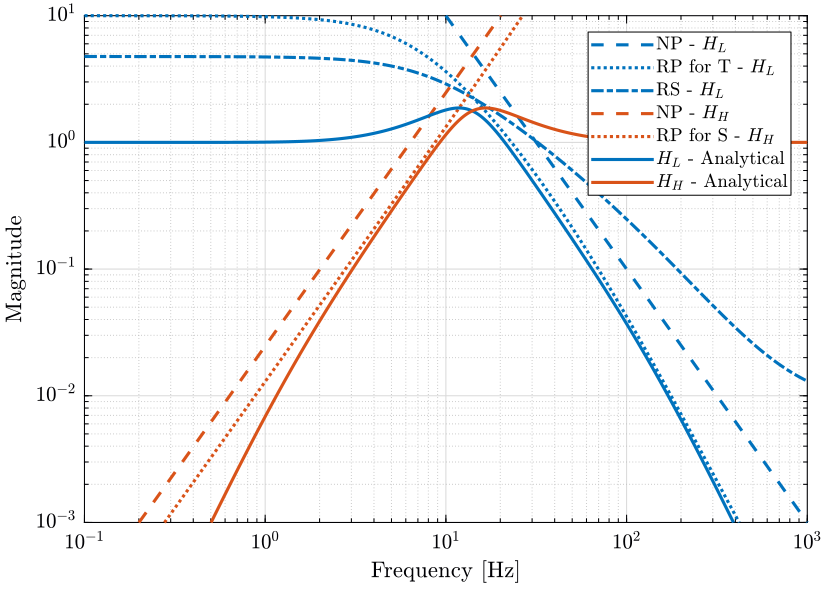
- Section 4: upper bounds on the magnitude of the complementary filters \(|H_L|\) and \(|H_H|\) are defined in order to ensure Nominal Performance (NP), Robust Stability (RS) and Robust Performance (RP)
- Then, \(H_L\) and \(H_H\) are synthesize such that \(|H_L|\) and \(|H_H|\) are within the specified bounds and such that \(H_L + H_H = 1\) (complementary property). This is done using two techniques, first \(\mathcal{H}_\infty\) (section 5) and then analytical formulas (section 6). Resulting complementary filters for both methods are compared in section 7.
- Section 8: the obtain controller \(K = G^{-1} H_H^{-1}\) is analyzed
- Section 9: the Nominal Stability (NS) and Nominal Performance conditions are verified
- Section 10: robust Stability and Robust Performance conditions are studied
- Section 11: a pre-filter that is used to limit the input usage due to the change of the reference is added
- Section 12: a controller is designed using
SISOTOOLand then compared with the previously generated controller
All the files (data and Matlab scripts) are accessible here.
1 Definition of the plant
The studied system consists of a solid positioned on top of a motorized uni-axial soft suspension.
The absolute position \(x\) of the solid is measured using an inertial sensor and a force \(F\) can be applied to the mass using a voice coil actuator.
The model of the system is represented on figure 2 where the mass of the solid is \(m = 20\ [kg]\), the stiffness of the suspension is \(k = 10^4\ [N/m]\) and the damping of the system is \(c = 10^2\ [N/(m/s)]\).

Figure 2: One degree of freedom system
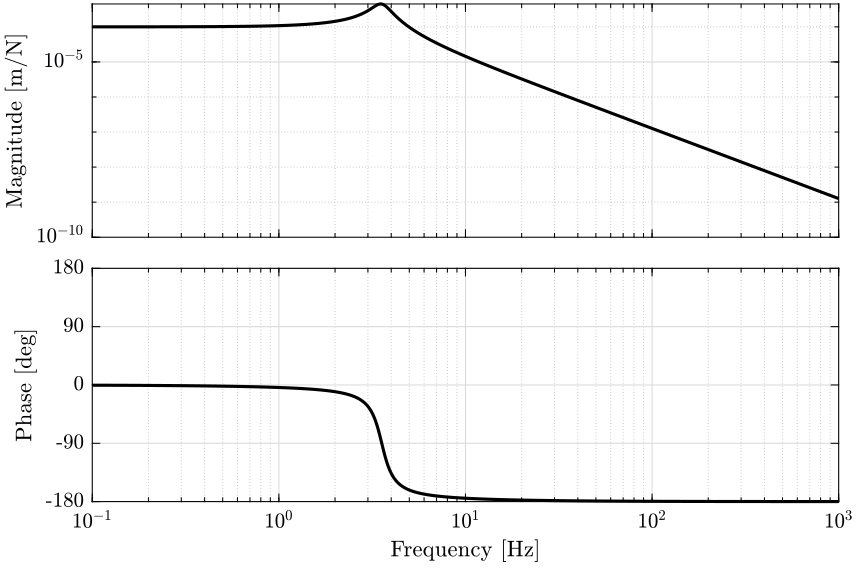
The plant \(G\) is defined on matlab and its bode plot is shown on figure 3.
m = 20;  % [kg]
k = 1e4; % [N/m]
c = 1e2; % [N/(m/s)]

G = 1/(m*s^2 + c*s + k);
2 Multiplicative input uncertainty
We choose to use the multiplicative input uncertainty to model the plant uncertainty: \[ \Pi_I: \ G^\prime(s) = G(s) (1 + w_I(s) \Delta(s)),\text{ with } |\Delta(j\omega)| < 1 \ \forall \omega \]
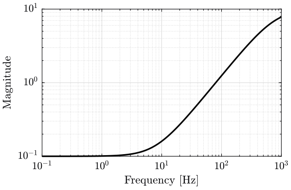
The uncertainty weight \(w_I\) has the following form: \[ w_I(s) = \frac{\tau s + r_0}{(\tau/r_\infty) s + 1} \] where \(r_0=0.1\) is the relative uncertainty at steady-state, \(1/\tau=80\text{Hz}\) is the frequency at which the relative uncertainty reaches 100%, and \(r_\infty=10\) is the magnitude of the weight at high frequency.
We defined the uncertainty weight on matlab. Its bode plot is shown on figure 4.
r0 = 0.1;
rinf = 10;
tau = 1/2/pi/80;

wI = (tau*s + r0)/((tau/rinf)*s+1);
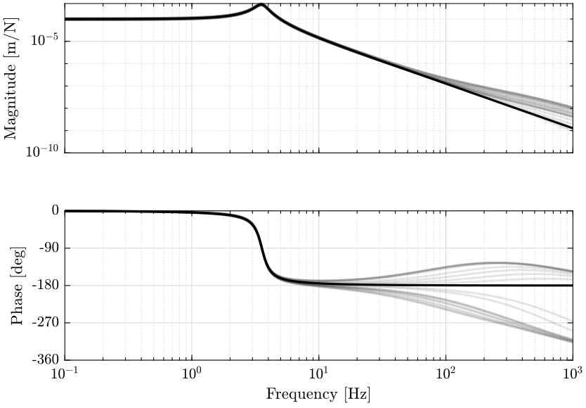
The uncertain model is created with the ultidyn function. Elements in the uncertainty set \(\Pi_I\) are computed and their bode plot is shown on figure 5.
Delta = ultidyn('Delta', [1 1]);

Gd = G*(1+wI*Delta);
Gds = usample(Gd, 20);
3 Specifications and performance weights
The control objective is to isolate the displacement \(x\) of the mass from the ground motion \(w\).
The specifications are described below:
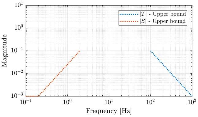
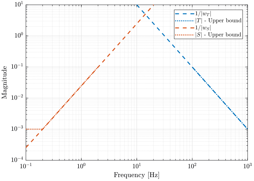
- at least a factor \(10\) of disturbance rejection at \(2\ \text{Hz}\) and with a slope of \(2\) below \(2\ \text{Hz}\) until a rejection of \(10^3\)
- the noise attenuation should be at least \(10\) above \(100\ \text{Hz}\) and with a slope of \(-2\) above
These specifications can be represented as upper bounds on the closed loop transfer functions \(S\) and \(T\) (see figure 6).
We now define two weights, \(w_S(s)\) and \(w_T(s)\) such that \(1/|w_S|\) and \(1/|w_T|\) are lower than the previously defined upper bounds. Then, the performance specifications are satisfied if the following condition is valid: \[ \big|S(j\omega)\big| < \frac{1}{|w_S(j\omega)|} ; \quad \big|T(j\omega)\big| < \frac{1}{|w_T(j\omega)|}, \quad \forall \omega \]
The weights are defined as follow. They magnitude is compared with the upper bounds on \(S\) and \(T\) on figure 7.
wS = 1600/(s+0.13)^2;
wT = 1000*((s/(2*pi*1000)))^2;
4 Upper bounds on the norm of the complementary filters for NP, RS and RP
Now that we have defined \(w_I\), \(w_S\) and \(w_T\), we can derive conditions for Nominal Performance, Robust Stability and Robust Performance (\(j\omega\) is omitted here for readability):
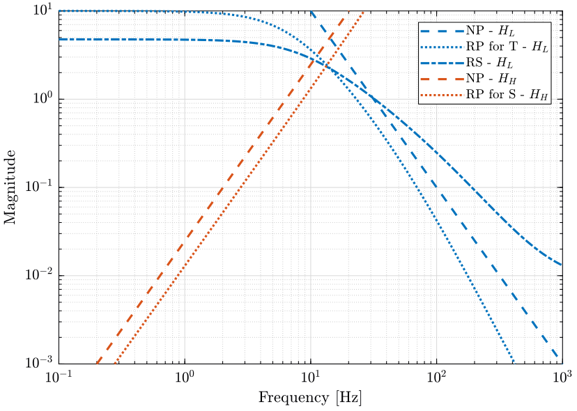
\begin{align*} \text{NP} &\Leftrightarrow |H_H| < \frac{1}{|w_S|} \text{ and } |H_L| < \frac{1}{|w_T|} \quad \forall \omega \\ \text{RS} &\Leftrightarrow |H_L| < \frac{1}{|w_I| (2 + |w_I|)} \quad \forall \omega \\ \text{RP for } S &\Leftarrow |H_H| < \frac{1 + |w_I|}{|w_S| (2 + |w_I|)} \quad \forall \omega \\ \text{RP for } T &\Leftrightarrow |H_L| < \frac{1}{|w_T| (1 + |w_I|) + |w_I|} \quad \forall \omega \end{align*}These conditions are upper bounds on the complementary filters used for control.
We plot these conditions on figure 8.
5 H-Infinity synthesis of complementary filters
We here synthesize the complementary filters using the \(\mathcal{H}_\infty\) synthesis. The goal is to specify upper bounds on the norms of \(H_L\) and \(H_H\) while ensuring their complementary property (\(H_L + H_H = 1\)).
In order to do so, we use the generalized plant shown on figure 9 where \(w_L\) and \(w_H\) weighting transfer functions that will be used to shape \(H_L\) and \(H_H\) respectively.

Figure 9: Generalized plant used for the \(\mathcal{H}_\infty\) synthesis of the complementary filters
The \(\mathcal{H}_\infty\) synthesis applied on this generalized plant will give a transfer function \(H_L\) (figure 10) such that the \(\mathcal{H}_\infty\) norm of the transfer function from \(w\) to \([z_H,\ z_L]\) is less than one: \[ \left\| \begin{array}{c} H_L w_L \\ (1 - H_L) w_H \end{array} \right\|_\infty < 1 \]
Thus, if the above condition is verified, we can define \(H_H = 1 - H_L\) and we have that: \[ \left\| \begin{array}{c} H_L w_L \\ H_H w_H \end{array} \right\|_\infty < 1 \] Which is almost (with an maximum error of \(\sqrt{2}\)) equivalent to:
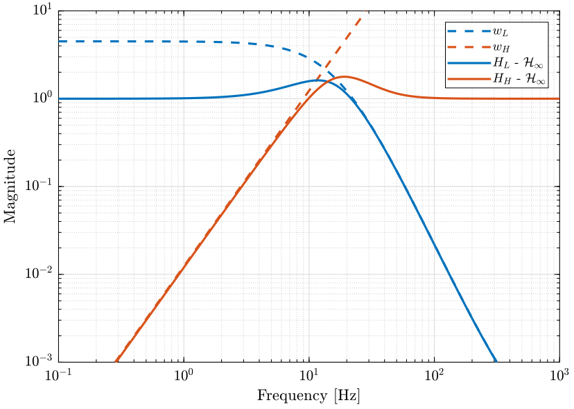
\begin{align*} |H_L| &< \frac{1}{|w_L|}, \quad \forall \omega \\ |H_H| &< \frac{1}{|w_H|}, \quad \forall \omega \end{align*}We then see that \(w_L\) and \(w_H\) can be used to shape both \(H_L\) and \(H_H\) while ensuring (by definition of \(H_H = 1 - H_L\)) their complementary property.

Figure 10: \(\mathcal{H}_\infty\) synthesis of the complementary filters
Thus, if we choose \(w_L\) and \(w_H\) such that \(1/|w_L|\) and \(1/|w_H|\) lie below the upper bounds of figure 8, we will ensure the NP, RS and RP of the controlled system.
Depending if we are interested only in NP, RS or RP, we can adjust the weights \(w_L\) and \(w_H\).
omegab = 2*pi*9;
wH = (omegab)^2/(s + omegab*sqrt(1e-5))^2;
omegab = 2*pi*28;
wL = (s + omegab/(4.5)^(1/3))^3/(s*(1e-4)^(1/3) + omegab)^3;
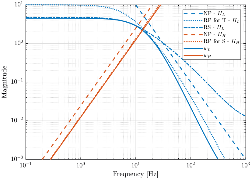
Figure 11: Weights on the complementary filters \(w_L\) and \(w_H\) and the associated performance weights (png, pdf)
We define the generalized plant \(P\) on matlab.
P = [0   wL;
     wH -wH;
     1   0];
And we do the \(\mathcal{H}_\infty\) synthesis using the hinfsyn command.
[Hl_hinf, ~, gamma, ~] = hinfsyn(P, 1, 1,'TOLGAM', 0.001, 'METHOD', 'ric', 'DISPLAY', 'on');
[Hl_hinf, ~, gamma, ~] = hinfsyn(P, 1, 1,'TOLGAM', 0.001, 'METHOD', 'ric', 'DISPLAY', 'on');
Test bounds:      0.0000 <  gamma  <=      1.7285

  gamma    hamx_eig  xinf_eig  hamy_eig   yinf_eig   nrho_xy   p/f
    1.729   4.1e+01   8.4e-12   1.8e-01    0.0e+00    0.0000    p
    0.864   3.9e+01 -5.8e-02#  1.8e-01    0.0e+00    0.0000    f
    1.296   4.0e+01   8.4e-12   1.8e-01    0.0e+00    0.0000    p
    1.080   4.0e+01   8.5e-12   1.8e-01    0.0e+00    0.0000    p
    0.972   3.9e+01 -4.2e-01#  1.8e-01    0.0e+00    0.0000    f
    1.026   4.0e+01   8.5e-12   1.8e-01    0.0e+00    0.0000    p
    0.999   3.9e+01   8.5e-12   1.8e-01    0.0e+00    0.0000    p
    0.986   3.9e+01 -1.2e+00#  1.8e-01    0.0e+00    0.0000    f
    0.993   3.9e+01 -8.2e+00#  1.8e-01    0.0e+00    0.0000    f
    0.996   3.9e+01   8.5e-12   1.8e-01    0.0e+00    0.0000    p
    0.994   3.9e+01   8.5e-12   1.8e-01    0.0e+00    0.0000    p
    0.993   3.9e+01 -3.2e+01#  1.8e-01    0.0e+00    0.0000    f

 Gamma value achieved:     0.9942
We then define the high pass filter \(H_H = 1 - H_L\). The bode plot of both \(H_L\) and \(H_H\) is shown on figure 12.
Hh_hinf = 1 - Hl_hinf;
6 Complementary filters using analytical formula
We here use analytical formula for the complementary filters \(H_L\) and \(H_H\).
The first two formulas that are used to generate complementary filters are:
\begin{align*} H_L(s) &= \frac{(1+\alpha) (\frac{s}{\omega_0})+1}{\left((\frac{s}{\omega_0})+1\right) \left((\frac{s}{\omega_0})^2 + \alpha (\frac{s}{\omega_0}) + 1\right)}\\ H_H(s) &= \frac{(\frac{s}{\omega_0})^2 \left((\frac{s}{\omega_0})+1+\alpha\right)}{\left((\frac{s}{\omega_0})+1\right) \left((\frac{s}{\omega_0})^2 + \alpha (\frac{s}{\omega_0}) + 1\right)} \end{align*}where:
- \(\omega_0\) is the blending frequency in rad/s.
- \(\alpha\) is used to change the shape of the filters:
- Small values for \(\alpha\) will produce high magnitude of the filters \(|H_L(j\omega)|\) and \(|H_H(j\omega)|\) near \(\omega_0\) but smaller value for \(|H_L(j\omega)|\) above \(\approx 1.5 \omega_0\) and for \(|H_H(j\omega)|\) below \(\approx 0.7 \omega_0\)
- A large \(\alpha\) will do the opposite
This is illustrated on figure 13. As it is usually wanted to have the \(\| S \|_\infty < 2\), \(\alpha\) between \(0.5\) and \(1\) gives a good trade-off between the performance and the robustness. The slope of those filters at high and low frequencies is \(-2\) and \(2\) respectively for \(H_L\) and \(H_H\).
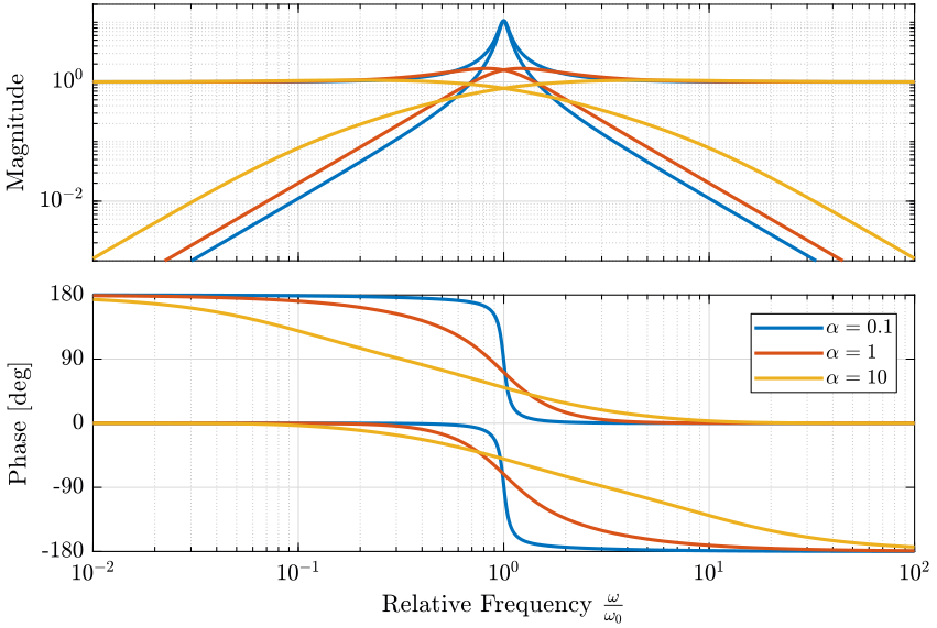
Figure 13: Effect of the parameter \(\alpha\) on the shape of the generated second order complementary filters (png, pdf)
The parameters \(\alpha\) and \(\omega_0\) are chosen in order to have that the complementary filters stay below the defined upper bounds.
The obtained complementary filters are shown on figure 14. The Robust Performance is not fulfilled for \(T\), and we see that the RP condition as a slop of \(-3\). We thus have to use different formula for the complementary filters here.
w0 = 2*pi*13;
alpha = 0.8;

Hh2_ana = (s/w0)^2*((s/w0)+1+alpha)/(((s/w0)+1)*((s/w0)^2 + alpha*(s/w0) + 1));
Hl2_ana = ((1+alpha)*(s/w0)+1)/(((s/w0)+1)*((s/w0)^2 + alpha*(s/w0) + 1));
The following formula gives complementary filters with slopes of \(-3\) and \(3\):
\begin{align*} H_L(s) &= \frac{\left(1+(\alpha+1)(\beta+1)\right) (\frac{s}{\omega_0})^2 + (1+\alpha+\beta)(\frac{s}{\omega_0}) + 1}{\left(\frac{s}{\omega_0} + 1\right) \left( (\frac{s}{\omega_0})^2 + \alpha (\frac{s}{\omega_0}) + 1 \right) \left( (\frac{s}{\omega_0})^2 + \beta (\frac{s}{\omega_0}) + 1 \right)}\\ H_H(s) &= \frac{(\frac{s}{\omega_0})^3 \left( (\frac{s}{\omega_0})^2 + (1+\alpha+\beta) (\frac{s}{\omega_0}) + (1+(\alpha+1)(\beta+1)) \right)}{\left(\frac{s}{\omega_0} + 1\right) \left( (\frac{s}{\omega_0})^2 + \alpha (\frac{s}{\omega_0}) + 1 \right) \left( (\frac{s}{\omega_0})^2 + \beta (\frac{s}{\omega_0}) + 1 \right)} \end{align*}The parameters are:
- \(\omega_0\) is the blending frequency in rad/s
- \(\alpha\) and \(\beta\) that are used to change the shape of the filters similarly to the parameter \(\alpha\) for the second order complementary filters
The filters are defined below and the result is shown on figure 15 where we can see that the complementary filters are below the defined upper bounds.
alpha = 1;
beta = 10;
w0 = 2*pi*14;

Hh3_ana = (s/w0)^3 * ((s/w0)^2 + (1+alpha+beta)*(s/w0) + (1+(alpha+1)*(beta+1)))/((s/w0 + 1)*((s/w0)^2+alpha*(s/w0)+1)*((s/w0)^2+beta*(s/w0)+1));
Hl3_ana = ((1+(alpha+1)*(beta+1))*(s/w0)^2 + (1+alpha+beta)*(s/w0) + 1)/((s/w0 + 1)*((s/w0)^2+alpha*(s/w0)+1)*((s/w0)^2+beta*(s/w0)+1));
7 Comparison of complementary filters
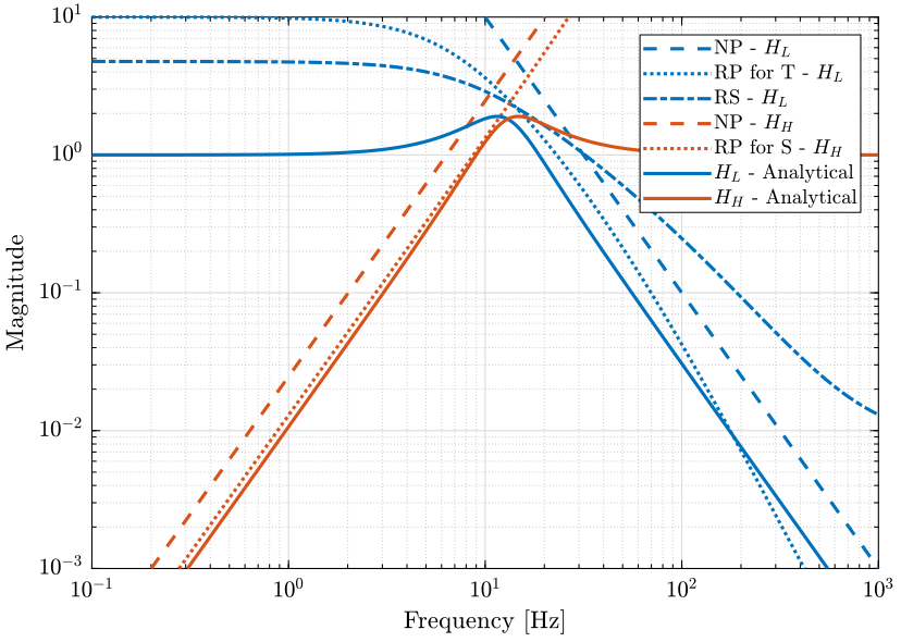
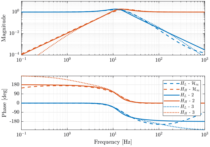
The generated complementary filters using \(\mathcal{H}_\infty\) and the analytical formulas are compared on figure 16.
Although they are very close to each other, there is some difference to note here:
- the analytical formula provides a very simple way to generate the complementary filters (and thus the controller), they could even be used to tune the controller online using the parameters \(\alpha\) and \(\omega_0\). However, these formula have the property that \(|H_H|\) and \(|H_L|\) are symmetrical with the frequency \(\omega_0\) which may not be desirable.
- while the \(\mathcal{H}_\infty\) synthesis of the complementary filters is not as straightforward as using the analytical formula, it provides a more optimized procedure to obtain the complementary filters
The complementary filters obtained with the \(\mathcal{H}_\infty\) will be used for further analysis.
8 Controller Analysis
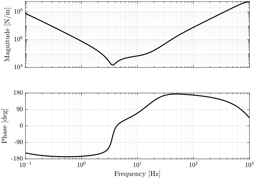
The controller \(K\) is computed from the plant model \(G\) and the low pass filter \(H_H\): \[ K = G^{-1} H_H^{-1} \]
As this is not proper and thus realizable, a second order low pass filter is added with a crossover frequency much larger than the control bandwidth.
omega = 2*pi*1000;
K = 1/(Hh_hinf*G) * 1/((1+s/omega)*(1+s/omega+(s/omega)^2));
zpk(K)

ans =

        4.961e12 (s+9.915e04) (s^2 + 5s + 500) (s^2 + 284.6s + 2.135e04) (s^2 + 130.5s + 9887)
  --------------------------------------------------------------------------------------------------
  (s+9.914e04) (s+6283) (s^2 + 0.3576s + 0.03198) (s^2 + 413.8s + 6.398e04) (s^2 + 6283s + 3.948e07)

Continuous-time zero/pole/gain model.
The bode plot of the controller is shown on figure 17:
- two integrator are present at low frequency
- the resonance of the plant at \(3.5\ \text{Hz}\) is inverted (notched)
- a lead is added at \(10\ \text{Hz}\)
9 Nominal Stability and Nominal Performance
The nominal stability of the system is first checked with the allmargin matlab command.
allmargin(K*G*Hl_hinf)
allmargin(K*G*Hl_hinf)
ans =
  struct with fields:

     GainMargin: 4.46426896164391
    GMFrequency: 243.854595348016
    PhaseMargin: 35.7045152899792
    PMFrequency: 88.3664383511655
    DelayMargin: 0.00705201387841809
    DMFrequency: 88.3664383511655
         Stable: 1
The system is stable and the stability margins are good.
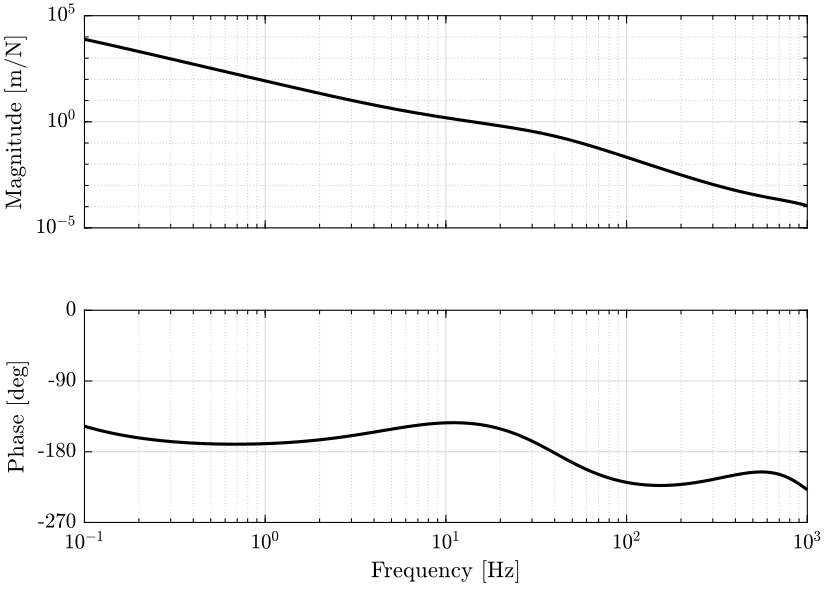
The bode plot of the loop gain \(L = K*G*H_L\) is shown on figure 18.
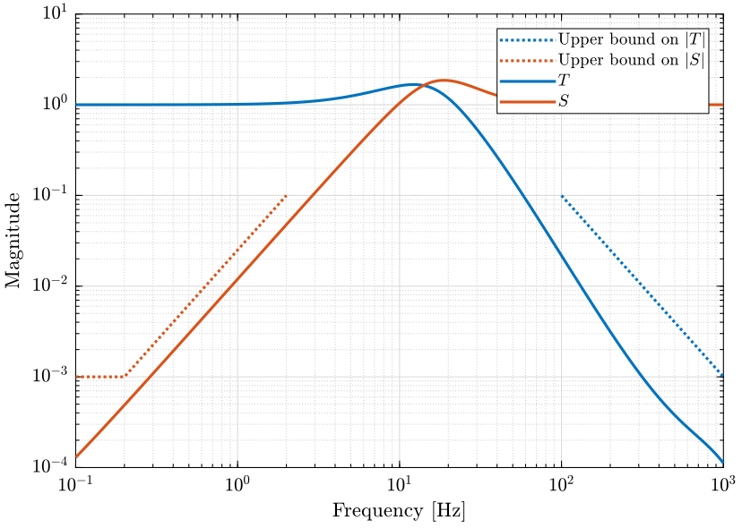
In order to check the Nominal Performance of the system, we compute the sensibility and the complementary sensibility transfer functions.
S = 1/(K*G*Hl_hinf + 1);
T = K*G*Hl_hinf/(K*G*Hl_hinf + 1);
We then compare their norms with the upper bounds on the performance of the system (figure 19). As expected, we guarantee the Nominal Performance of the system.
10 Robust Stability and Robust Performance
In order to verify the Robust stability of the system, we can use the following equivalence: \[ \text{RS} \Leftrightarrow \left| w_I T \right| < 1 \quad \forall \omega \]
This is shown on figure 20.
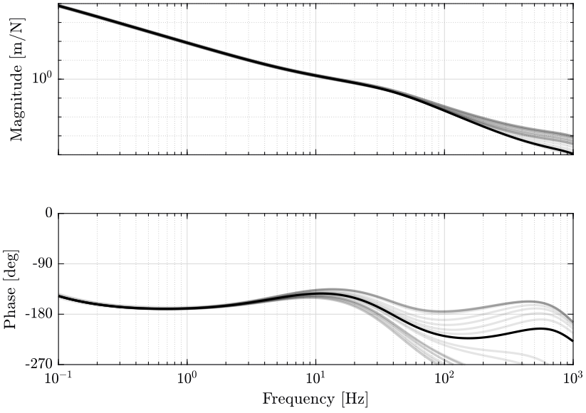
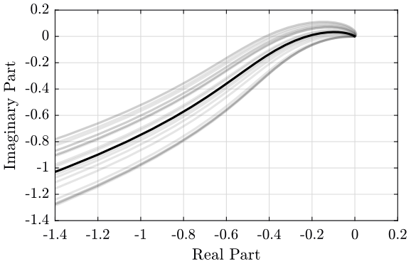
To check Robust Stability, we can also look at the loop gain of the uncertain system (figure 21) or the Nyquist plot (figure 22).
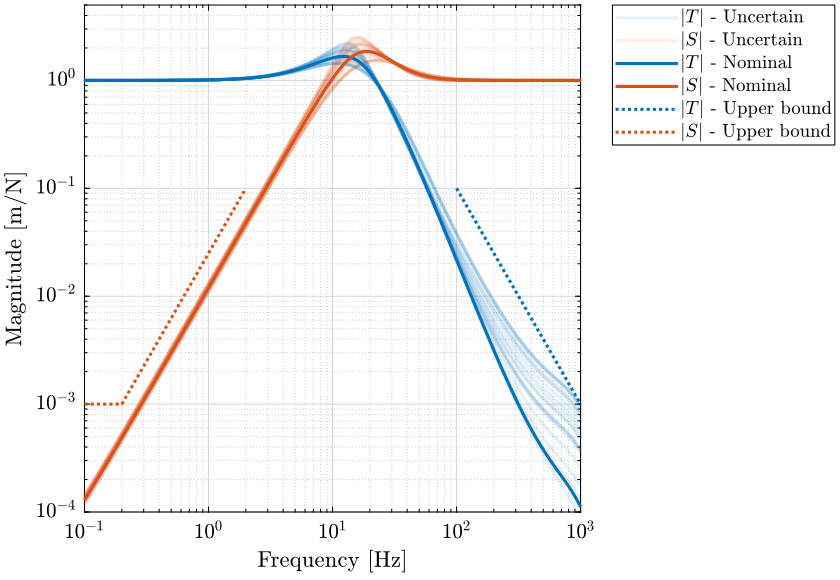
The Robust Performance is verified by plotting \(|S|\) and \(|T|\) for the uncertain system along side the upper bounds defined for performance. This is shown on figure 23 and we can indeed confirmed that the robust performance property of the system is valid.
11 Pre-filter
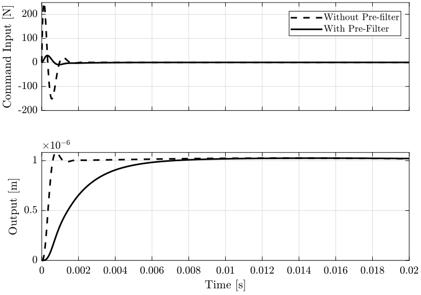
For now, we have not specified any performance requirements on the input usage due to change of reference. Do limit the input usage due to change of reference, we can use a pre-filter \(K_r\) as shown on figure 1.
If we want a response time of 0.01 second, we can choose a first order low pass filter with a crossover frequency at \(1/0.01 = 100\ \text{Hz}\) as defined below.
Kr = 1/(1+s/2/pi/100);
We then run a simulation for a step of \(1\mu m\) for the system without and with the pre-filter \(K_r\) (figure 24). This confirms that a pre-filter can be used to limit the input usage due to change of reference using this architecture.
t  = linspace(0, 0.02, 1000);

opts = stepDataOptions;
opts.StepAmplitude = 1e-6;

u  = step((K)/(1+G*K*Hl_hinf),      t, opts);
uf = step((Kr*K)/(1+G*K*Hl_hinf),   t, opts);
y  = step((K*G)/(1+G*K*Hl_hinf),    t, opts);
yf = step((Kr*G*K)/(1+G*K*Hl_hinf), t, opts);
12 Controller using classical techniques
A controller is designed using SISOTOOL with a bandwidth of approximately \(20\ \text{Hz}\) and with two integrator.
The obtained controller is shown below.
Kf = 1.1814e12*(s+10.15)*(s+9.036)*(s+53.8)/(s^2*(s+216.1)*(s+1200)*(s+1864));
zpk(Kf)
zpk(Kf)

ans =

  1.1814e12 (s+10.15) (s+9.036) (s+53.8)
  --------------------------------------
     s^2 (s+216.1) (s+1200) (s+1864)

Continuous-time zero/pole/gain model.
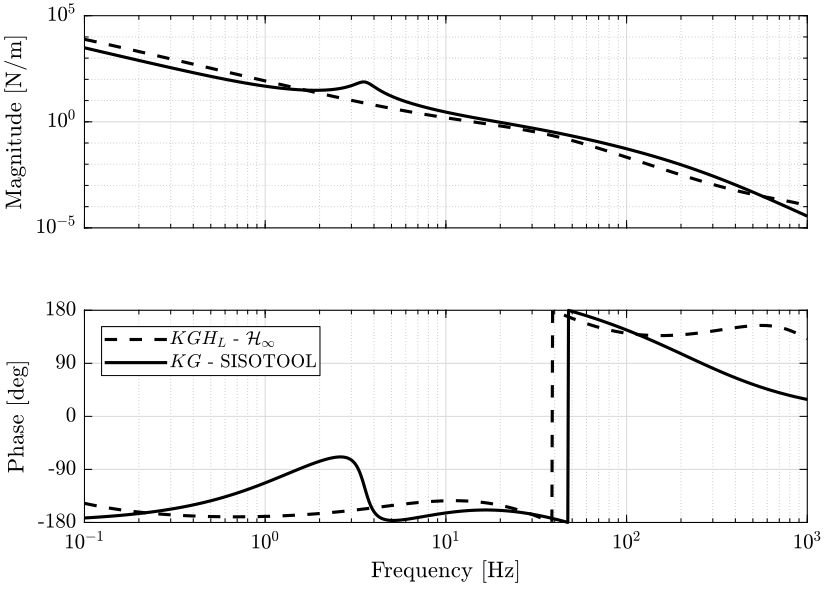
The loop gain for both cases are compared on figure 25.
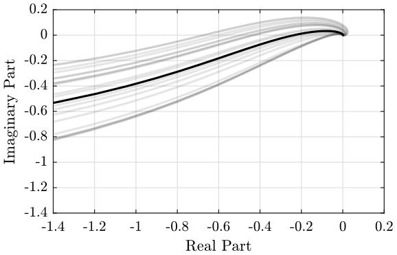
The Robust Stability of the system is verified using the Nyquist plot on figure 26.
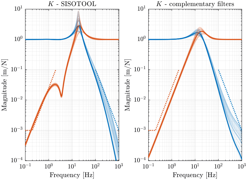
The closed loop sensitivity and complementary sensitivity transfer functions are computed. And finally, the Robust Performance of both systems are compared on figure 27.
