Robust and Optimal Sensor Fusion - Matlab Computation
Table of Contents
- 1. Optimal Super Sensor Noise: \(\mathcal{H}_2\) Synthesis
- 2. Robust Sensor Fusion: \(\mathcal{H}_\infty\) Synthesis
- 2.1. Super Sensor Dynamical Uncertainty
- 2.2. Dynamical uncertainty of the individual sensors
- 2.3. Synthesis objective
- 2.4. Requirements as an \(\mathcal{H}_\infty\) norm
- 2.5. Weighting Function used to bound the super sensor uncertainty
- 2.6. \(\mathcal{H}_\infty\) Synthesis
- 2.7. Super sensor uncertainty
- 2.8. Super sensor noise
- 2.9. Conclusion
- 3. Optimal and Robust Sensor Fusion: Mixed \(\mathcal{H}_2/\mathcal{H}_\infty\) Synthesis
- 3.1. Mixed \(\mathcal{H}_2\) / \(\mathcal{H}_\infty\) Synthesis - Introduction
- 3.2. Noise characteristics and Uncertainty of the individual sensors
- 3.3. Weighting Functions on the uncertainty of the super sensor
- 3.4. Mixed Synthesis Architecture
- 3.5. Mixed \(\mathcal{H}_2\) / \(\mathcal{H}_\infty\) Synthesis
- 3.6. Obtained Super Sensor’s noise
- 3.7. Obtained Super Sensor’s Uncertainty
- 3.8. Conclusion
In this document, the optimal and robust design of complementary filters is studied.
Two sensors are considered with both different noise characteristics and dynamical uncertainties represented by multiplicative input uncertainty.
- Section 1: the \(\mathcal{H}_2\) synthesis is used to design complementary filters such that the RMS value of the super sensor’s noise is minimized
- Section 2: the \(\mathcal{H}_\infty\) synthesis is used to design complementary filters such that the super sensor’s uncertainty is bonded to acceptable values
- Section 3: the mixed \(\mathcal{H}_2/\mathcal{H}_\infty\) synthesis is used to both limit the super sensor’s uncertainty and to lower the RMS value of the super sensor’s noise
1 Optimal Super Sensor Noise: \(\mathcal{H}_2\) Synthesis
The idea is to combine sensors that works in different frequency range using complementary filters.
Doing so, one “super sensor” is obtained that can have better noise characteristics than the individual sensors over a large frequency range.
The complementary filters have to be designed in order to minimize the effect noise of each sensor on the super sensor noise.
The Matlab scripts is accessible here.
1.1 Architecture
Let’s consider the sensor fusion architecture shown on figure 1 where two sensors (sensor 1 and sensor 2) are measuring the same quantity \(x\) with different noise characteristics determined by \(N_1(s)\) and \(N_2(s)\).
\(\tilde{n}_1\) and \(\tilde{n}_2\) are normalized white noise:
\begin{equation} \label{orga7ad7f8} \Phi_{\tilde{n}_1}(\omega) = \Phi_{\tilde{n}_2}(\omega) = 1 \end{equation}
Figure 1: Fusion of two sensors
We consider that the two sensor dynamics \(G_1(s)\) and \(G_2(s)\) are ideal:
\begin{equation} \label{org024c8f5} G_1(s) = G_2(s) = 1 \end{equation}We obtain the architecture of figure 2.

Figure 2: Fusion of two sensors with ideal dynamics
\(H_1(s)\) and \(H_2(s)\) are complementary filters:
\begin{equation} \label{orga71be68} H_1(s) + H_2(s) = 1 \end{equation}The goal is to design \(H_1(s)\) and \(H_2(s)\) such that the effect of the noise sources \(\tilde{n}_1\) and \(\tilde{n}_2\) has the smallest possible effect on the estimation \(\hat{x}\).
We have that the Power Spectral Density (PSD) of \(\hat{x}\) is: \[ \Phi_{\hat{x}}(\omega) = |H_1(j\omega) N_1(j\omega)|^2 \Phi_{\tilde{n}_1}(\omega) + |H_2(j\omega) N_2(j\omega)|^2 \Phi_{\tilde{n}_2}(\omega), \quad \forall \omega \]
And the goal is the minimize the Root Mean Square (RMS) value of \(\hat{x}\):
\begin{equation} \label{orgc926b79} \sigma_{\hat{x}} = \sqrt{\int_0^\infty \Phi_{\hat{x}}(\omega) d\omega} \end{equation}1.2 Noise of the sensors
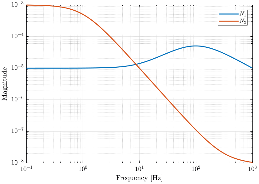
Let’s define the noise characteristics of the two sensors by choosing \(N_1\) and \(N_2\):
- Sensor 1 characterized by \(N_1(s)\) has low noise at low frequency (for instance a geophone)
- Sensor 2 characterized by \(N_2(s)\) has low noise at high frequency (for instance an accelerometer)
omegac = 100*2*pi; G0 = 1e-5; Ginf = 1e-4;
N1 = (Ginf*s/omegac + G0)/(s/omegac + 1)/(1 + s/2/pi/100);

omegac = 1*2*pi; G0 = 1e-3; Ginf = 1e-8;
N2 = ((sqrt(Ginf)*s/omegac + sqrt(G0))/(s/omegac + 1))^2/(1 + s/2/pi/4000)^2;
1.3 H-Two Synthesis
As \(\tilde{n}_1\) and \(\tilde{n}_2\) are normalized white noise: \(\Phi_{\tilde{n}_1}(\omega) = \Phi_{\tilde{n}_2}(\omega) = 1\) and we have: \[ \sigma_{\hat{x}} = \sqrt{\int_0^\infty |H_1 N_1|^2(\omega) + |H_2 N_2|^2(\omega) d\omega} = \left\| \begin{matrix} H_1 N_1 \\ H_2 N_2 \end{matrix} \right\|_2 \] Thus, the goal is to design \(H_1(s)\) and \(H_2(s)\) such that \(H_1(s) + H_2(s) = 1\) and such that \(\left\| \begin{matrix} H_1 N_1 \\ H_2 N_2 \end{matrix} \right\|_2\) is minimized.
For that, we use the \(\mathcal{H}_2\) Synthesis.
We use the generalized plant architecture shown on figure 4.

Figure 4: \(\mathcal{H}_2\) Synthesis - Generalized plant used for the optimal generation of complementary filters
The transfer function from \([n_1, n_2]\) to \(\hat{x}\) is: \[ \begin{bmatrix} N_1 H_1 \\ N_2 (1 - H_1) \end{bmatrix} \] If we define \(H_2 = 1 - H_1\), we obtain: \[ \begin{bmatrix} N_1 H_1 \\ N_2 H_2 \end{bmatrix} \]
Thus, if we minimize the \(\mathcal{H}_2\) norm of this transfer function, we minimize the RMS value of \(\hat{x}\).
We define the generalized plant \(P\) on matlab as shown on figure 4.
P = [0   N2  1;
     N1 -N2  0];
And we do the \(\mathcal{H}_2\) synthesis using the h2syn command.
[H1, ~, gamma] = h2syn(P, 1, 1);
Finally, we define \(H_2(s) = 1 - H_1(s)\).
H2 = 1 - H1;
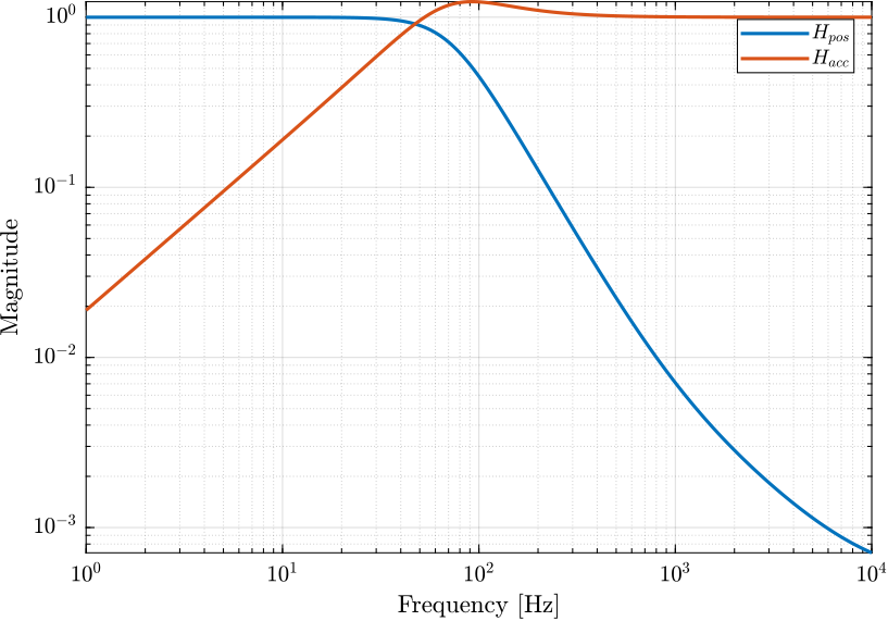
The complementary filters obtained are shown on figure 5.
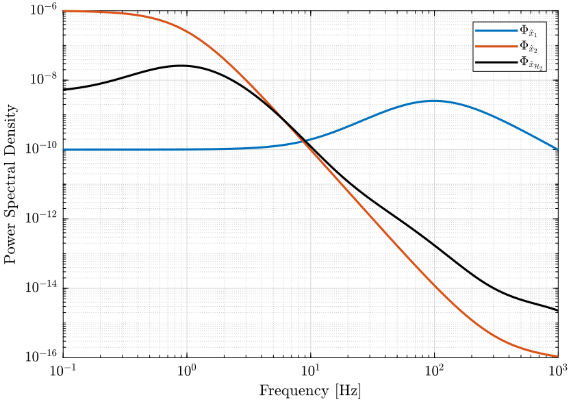
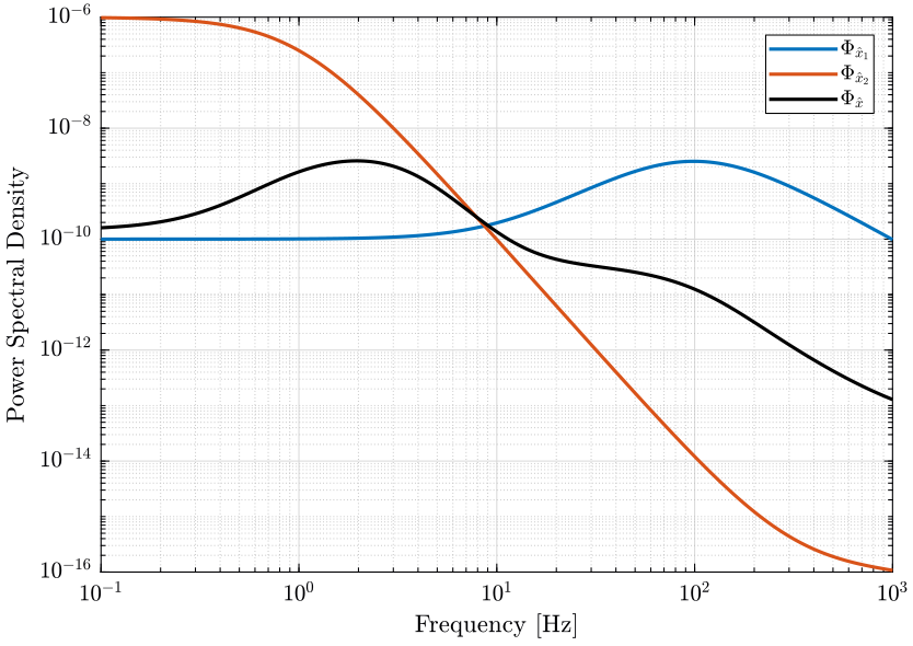
The PSD of the noise of the individual sensor and of the super sensor are shown in Fig. 6.
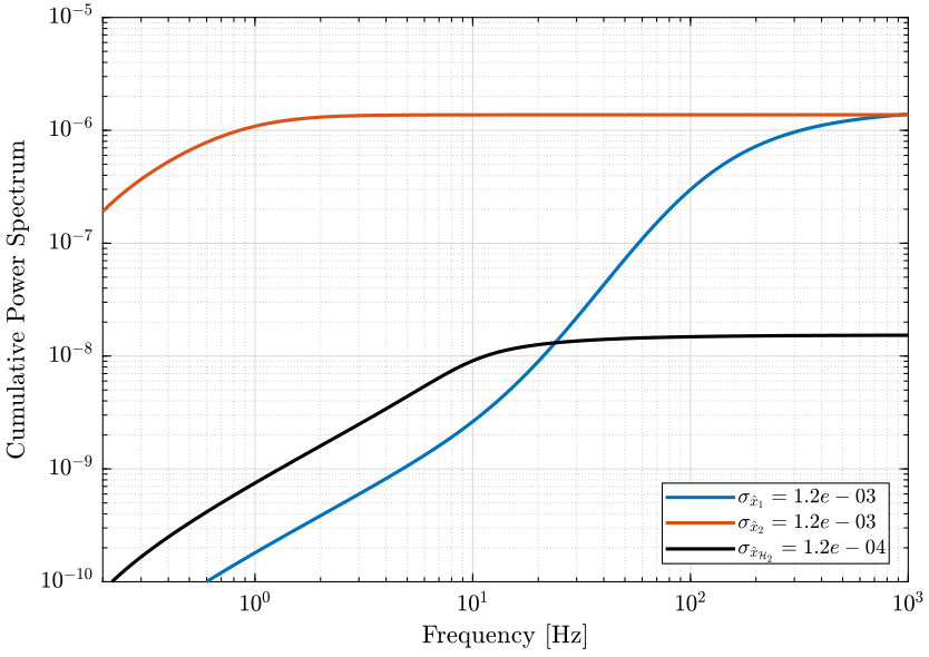
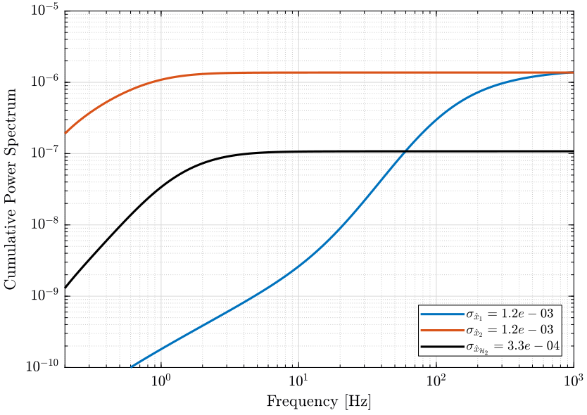
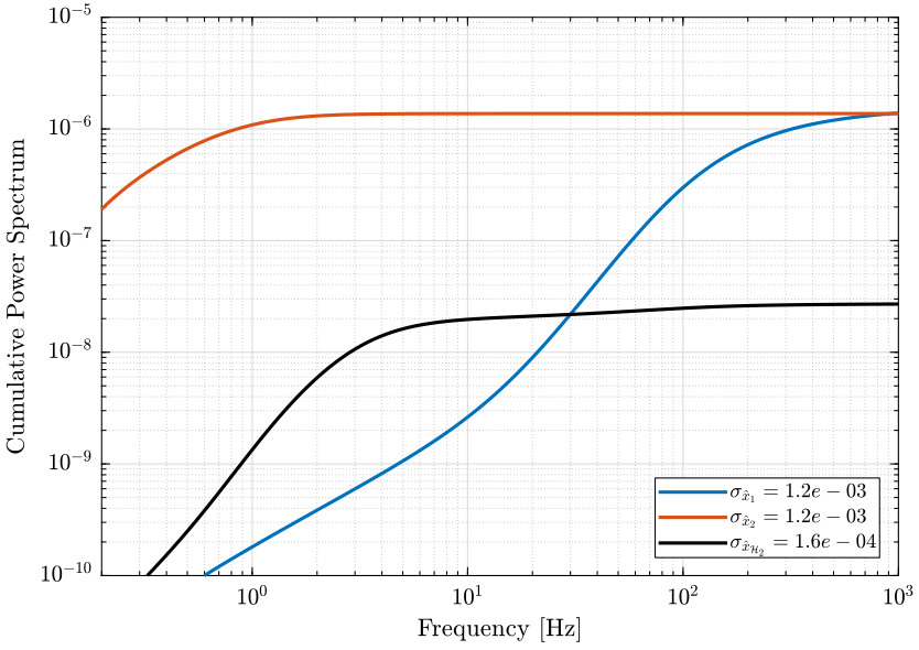
The Cumulative Power Spectrum (CPS) is shown on Fig. 7.
The obtained RMS value of the super sensor is lower than the RMS value of the individual sensors.
PSD_S1 = abs(squeeze(freqresp(N1, freqs, 'Hz'))).^2;
PSD_S2 = abs(squeeze(freqresp(N2, freqs, 'Hz'))).^2;
PSD_H2 = abs(squeeze(freqresp(N1*H1, freqs, 'Hz'))).^2+abs(squeeze(freqresp(N2*H2, freqs, 'Hz'))).^2;
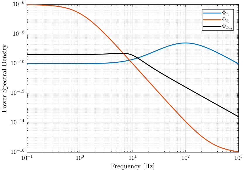
Figure 6: Power Spectral Density of the estimated \(\hat{x}\) using the two sensors alone and using the optimally fused signal (png, pdf)
CPS_S1 = 1/pi*cumtrapz(2*pi*freqs, PSD_S1);
CPS_S2 = 1/pi*cumtrapz(2*pi*freqs, PSD_S2);
CPS_H2 = 1/pi*cumtrapz(2*pi*freqs, PSD_H2);
1.4 Obtained Super Sensor’s noise uncertainty
We would like to verify if the obtained sensor fusion architecture is robust to change in the sensor dynamics.
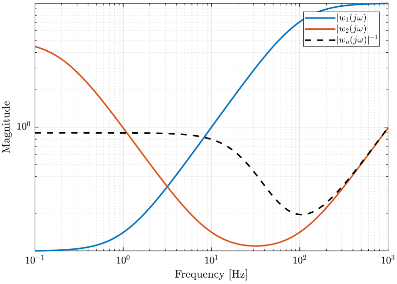
To study the dynamical uncertainty on the super sensor, we defined some multiplicative uncertainty on both sensor dynamics. Two weights \(w_1(s)\) and \(w_2(s)\) are used to described the amplitude of the dynamical uncertainty.
omegac = 100*2*pi; G0 = 0.1; Ginf = 10;
w1 = (Ginf*s/omegac + G0)/(s/omegac + 1);

omegac = 0.2*2*pi; G0 = 5; Ginf = 0.1;
w2 = (Ginf*s/omegac + G0)/(s/omegac + 1);
omegac = 5000*2*pi; G0 = 1; Ginf = 50;
w2 = w2*(Ginf*s/omegac + G0)/(s/omegac + 1);
The sensor uncertain models are defined below.
G1 = 1 + w1*ultidyn('Delta',[1 1]);
G2 = 1 + w2*ultidyn('Delta',[1 1]);
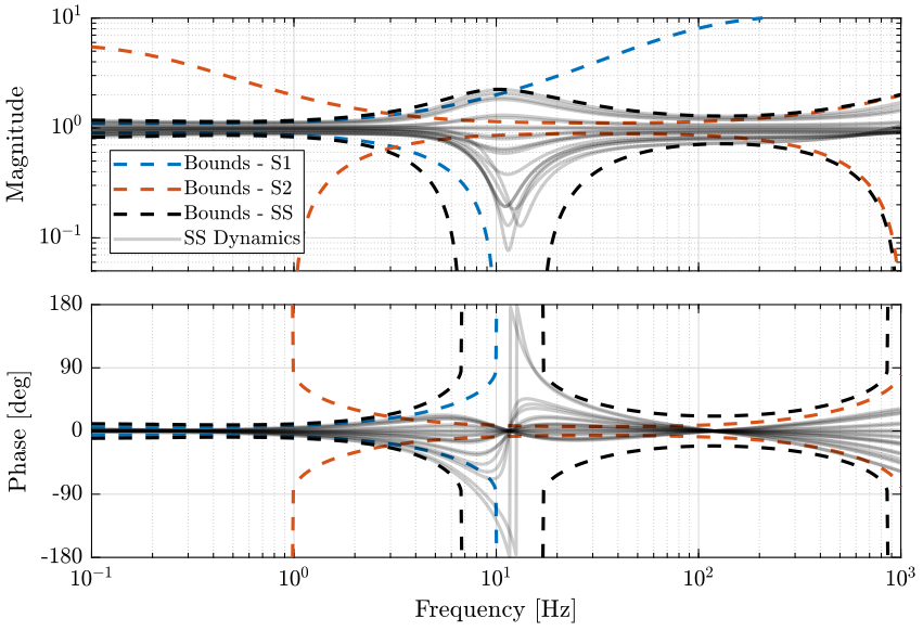
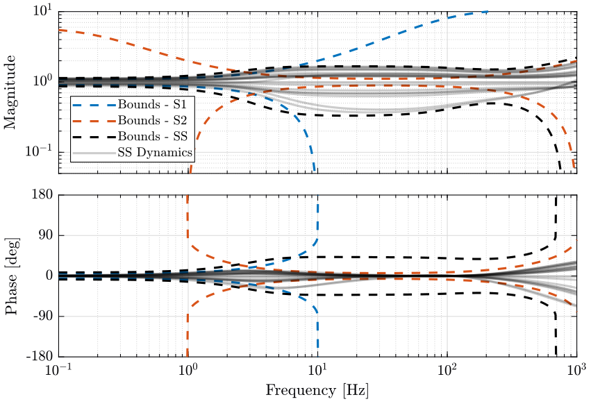
The super sensor uncertain model is defined below using the complementary filters obtained with the \(\mathcal{H}_2\) synthesis. The dynamical uncertainty bounds of the super sensor is shown in Fig. 8. Right Half Plane zero might be introduced in the super sensor dynamics which will render the feedback system unstable.
Gss = G1*H1 + G2*H2;
1.5 Conclusion
From the above complementary filter design with the \(\mathcal{H}_2\) and \(\mathcal{H}_\infty\) synthesis, it still seems that the \(\mathcal{H}_2\) synthesis gives the complementary filters that permits to obtain the minimal super sensor noise (when measuring with the \(\mathcal{H}_2\) norm).
However, the synthesis does not take into account the robustness of the sensor fusion.
2 Robust Sensor Fusion: \(\mathcal{H}_\infty\) Synthesis
We initially considered perfectly known sensor dynamics so that it can be perfectly inverted.
We now take into account the fact that the sensor dynamics is only partially known. To do so, we model the uncertainty that we have on the sensor dynamics by multiplicative input uncertainty as shown in Fig. 9.

Figure 9: Sensor fusion architecture with sensor dynamics uncertainty
The objective here is to design complementary filters \(H_1(s)\) and \(H_2(s)\) in order to minimize the dynamical uncertainty of the super sensor.
The Matlab scripts is accessible here.
2.1 Super Sensor Dynamical Uncertainty
In practical systems, the sensor dynamics has always some level of uncertainty. Let’s represent that with multiplicative input uncertainty as shown on figure 9.

Figure 10: Fusion of two sensors with input multiplicative uncertainty
The dynamics of the super sensor is represented by
\begin{align*} \frac{\hat{x}}{x} &= (1 + w_1 \Delta_1) H_1 + (1 + w_2 \Delta_2) H_2 \\ &= 1 + w_1 H_1 \Delta_1 + w_2 H_2 \Delta_2 \end{align*}with \(\Delta_i\) is any transfer function satisfying \(\| \Delta_i \|_\infty < 1\).
We see that as soon as we have some uncertainty in the sensor dynamics, we have that the complementary filters have some effect on the transfer function from \(x\) to \(\hat{x}\).
The uncertainty set of the transfer function from \(\hat{x}\) to \(x\) at frequency \(\omega\) is bounded in the complex plane by a circle centered on 1 and with a radius equal to \(|w_1(j\omega) H_1(j\omega)| + |w_2(j\omega) H_2(j\omega)|\) (figure 11).
We then have that the angle introduced by the super sensor is bounded by \(\arcsin(\epsilon)\): \[ \angle \frac{\hat{x}}{x}(j\omega) \le \arcsin \Big(|w_1(j\omega) H_1(j\omega)| + |w_2(j\omega) H_2(j\omega)|\Big) \]

Figure 11: Maximum phase variation
2.2 Dynamical uncertainty of the individual sensors
Let say we want to merge two sensors:
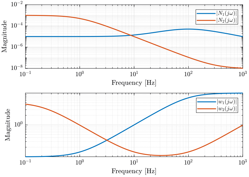
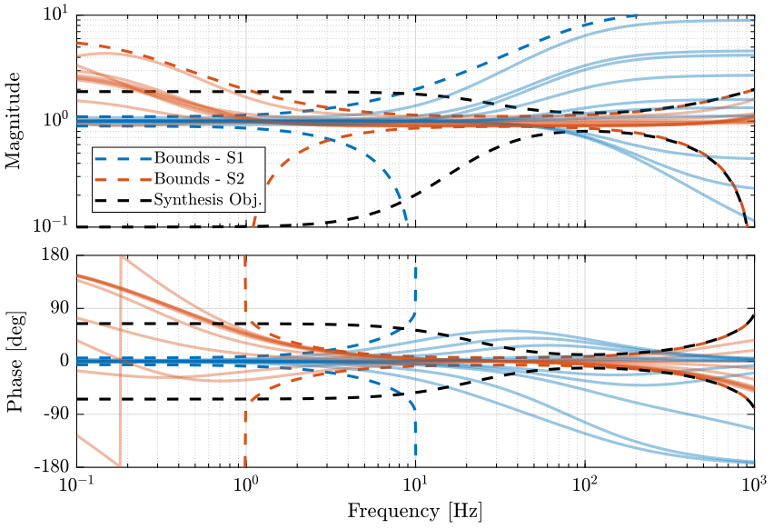
- sensor 1 that has unknown dynamics above 10Hz: \(|w_1(j\omega)| > 1\) for \(\omega > 10\text{ Hz}\)
- sensor 2 that has unknown dynamics below 1Hz and above 1kHz \(|w_2(j\omega)| > 1\) for \(\omega < 1\text{ Hz}\) and \(\omega > 1\text{ kHz}\)
We define the weights that are used to characterize the dynamic uncertainty of the sensors.
omegac = 100*2*pi; G0 = 0.1; Ginf = 10;
w1 = (Ginf*s/omegac + G0)/(s/omegac + 1);

omegac = 0.2*2*pi; G0 = 5; Ginf = 0.1;
w2 = (Ginf*s/omegac + G0)/(s/omegac + 1);
omegac = 5000*2*pi; G0 = 1; Ginf = 50;
w2 = w2*(Ginf*s/omegac + G0)/(s/omegac + 1);
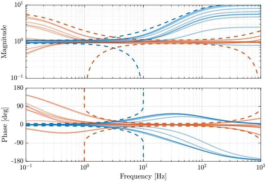
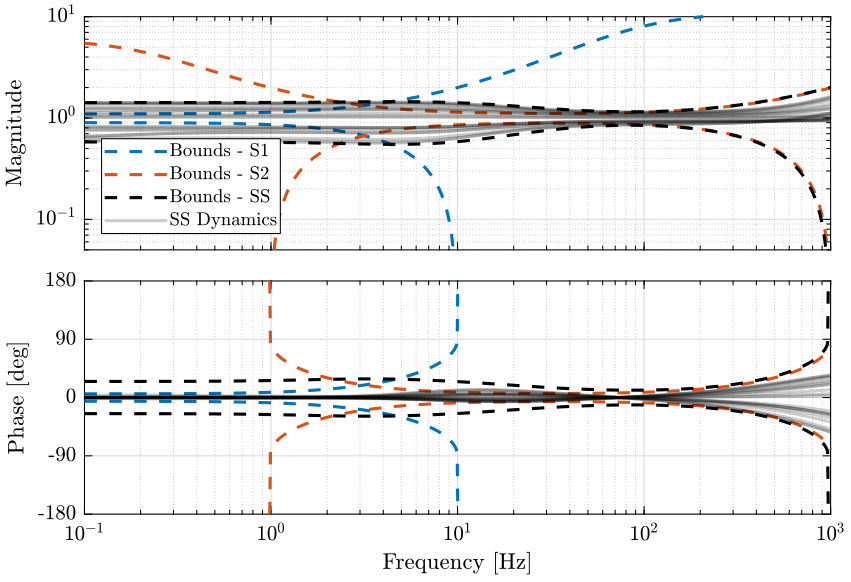
From the weights, we define the uncertain transfer functions of the sensors. Some of the uncertain dynamics of both sensors are shown on Fig. 12 with the upper and lower bounds on the magnitude and on the phase.
G1 = 1 + w1*ultidyn('Delta',[1 1]);
G2 = 1 + w2*ultidyn('Delta',[1 1]);
2.3 Synthesis objective
The uncertainty region of the super sensor dynamics is represented by a circle in the complex plane as shown in Fig. 11.
At each frequency \(\omega\), the radius of the circle is \(|w_1(j\omega) H_1(j\omega)| + |w_2(j\omega) H_2(j\omega)|\).
Thus, the phase shift \(\Delta\phi(\omega)\) due to the super sensor uncertainty is bounded by: \[ |\Delta\phi(\omega)| \leq \arcsin\big( |w_1(j\omega) H_1(j\omega)| + |w_2(j\omega) H_2(j\omega)| \big) \]
Let’s define some allowed frequency depend phase shift \(\Delta\phi_\text{max}(\omega) > 0\) such that: \[ |\Delta\phi(\omega)| < \Delta\phi_\text{max}(\omega), \quad \forall\omega \]
If \(H_1(s)\) and \(H_2(s)\) are designed such that \[ |w_1(j\omega) H_1(j\omega)| + |w_2(j\omega) H_2(j\omega)| < \sin\big( \Delta\phi_\text{max}(\omega) \big) \]
The maximum phase shift due to dynamic uncertainty at frequency \(\omega\) will be \(\Delta\phi_\text{max}(\omega)\).
2.4 Requirements as an \(\mathcal{H}_\infty\) norm
We now try to express this requirement in terms of an \(\mathcal{H}_\infty\) norm.
Let’s define one weight \(w_\phi(s)\) that represents the maximum wanted phase uncertainty: \[ |w_{\phi}(j\omega)|^{-1} \approx \sin(\Delta\phi_{\text{max}}(\omega)), \quad \forall\omega \]
Then:
\begin{align*} & |w_1(j\omega) H_1(j\omega)| + |w_2(j\omega) H_2(j\omega)| < \sin\big( \Delta\phi_\text{max}(\omega) \big), \quad \forall\omega \\ \Longleftrightarrow & |w_1(j\omega) H_1(j\omega)| + |w_2(j\omega) H_2(j\omega)| < |w_\phi(j\omega)|^{-1}, \quad \forall\omega \\ \Longleftrightarrow & \left| w_1(j\omega) H_1(j\omega) w_\phi(j\omega) \right| + \left| w_2(j\omega) H_2(j\omega) w_\phi(j\omega) \right| < 1, \quad \forall\omega \end{align*}Which is approximately equivalent to (with an error of maximum \(\sqrt{2}\)):
\begin{equation} \label{org559e8db} \left\| \begin{matrix} w_1(s) w_\phi(s) H_1(s) \\ w_2(s) w_\phi(s) H_2(s) \end{matrix} \right\|_\infty < 1 \end{equation}One should not forget that at frequency where both sensors has unknown dynamics (\(|w_1(j\omega)| > 1\) and \(|w_2(j\omega)| > 1\)), the super sensor dynamics will also be unknown and the phase uncertainty cannot be bounded. Thus, at these frequencies, \(|w_\phi|\) should be smaller than \(1\).
2.5 Weighting Function used to bound the super sensor uncertainty
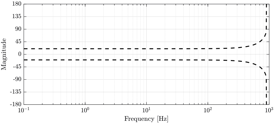
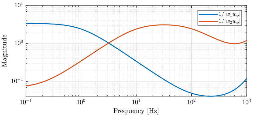
Let’s define \(w_\phi(s)\) in order to bound the maximum allowed phase uncertainty \(\Delta\phi_\text{max}\) of the super sensor dynamics. The magnitude \(|w_\phi(j\omega)|\) is shown in Fig. 13 and the corresponding maximum allowed phase uncertainty of the super sensor dynamics of shown in Fig. 14.
Dphi = 20; % [deg]

n = 4; w0 = 2*pi*900; G0 = 1/sin(Dphi*pi/180); Ginf = 1/100; Gc = 1;
wphi = (((1/w0)*sqrt((1-(G0/Gc)^(2/n))/(1-(Gc/Ginf)^(2/n)))*s + (G0/Gc)^(1/n))/((1/Ginf)^(1/n)*(1/w0)*sqrt((1-(G0/Gc)^(2/n))/(1-(Gc/Ginf)^(2/n)))*s + (1/Gc)^(1/n)))^n;

W1 = w1*wphi;
W2 = w2*wphi;
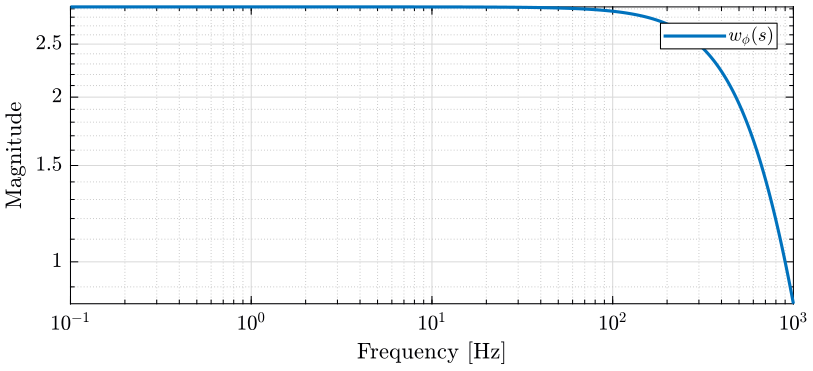
Figure 13: Magnitude of the weght \(w_\phi(s)\) that is used to bound the uncertainty of the super sensor (png, pdf)
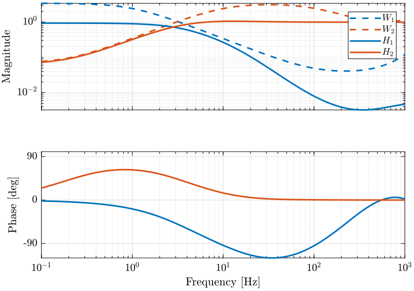
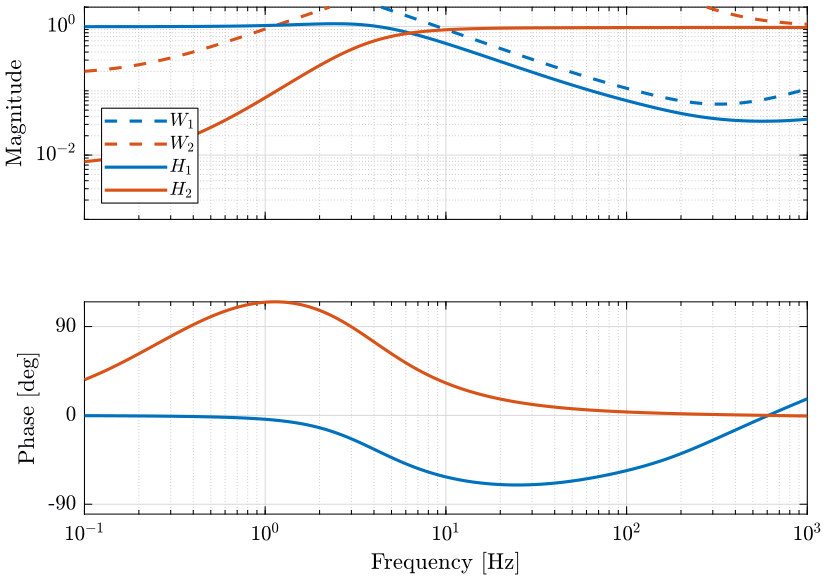
The obtained upper bounds on the complementary filters in order to limit the phase uncertainty of the super sensor are represented in Fig. 15.
2.6 \(\mathcal{H}_\infty\) Synthesis
The \(\mathcal{H}_\infty\) synthesis architecture used for the complementary filters is shown in Fig. 16.

Figure 16: Architecture used for \(\mathcal{H}_\infty\) synthesis of complementary filters
The generalized plant is defined below.
P = [W1 -W1;
     0   W2;
     1   0];
And we do the \(\mathcal{H}_\infty\) synthesis using the hinfsyn command.
[H2, ~, gamma, ~] = hinfsyn(P, 1, 1,'TOLGAM', 0.001, 'METHOD', 'ric', 'DISPLAY', 'on');
[H2, ~, gamma, ~] = hinfsyn(P, 1, 1,'TOLGAM', 0.001, 'METHOD', 'ric', 'DISPLAY', 'on');
Resetting value of Gamma min based on D_11, D_12, D_21 terms

Test bounds:      0.0447 <  gamma  <=      1.3318

  gamma    hamx_eig  xinf_eig  hamy_eig   yinf_eig   nrho_xy   p/f
    1.332   1.3e+01 -1.0e-14   1.3e+00   -2.6e-18    0.0000    p
    0.688   1.3e-11# ********   1.3e+00   -6.7e-15  ********    f
    1.010   1.1e+01 -1.5e-14   1.3e+00   -2.5e-14    0.0000    p
    0.849   6.9e-11# ********   1.3e+00   -2.3e-14  ********    f
    0.930   5.2e-12# ********   1.3e+00   -6.1e-18  ********    f
    0.970   5.6e-11# ********   1.3e+00   -2.3e-14  ********    f
    0.990   5.0e-11# ********   1.3e+00   -1.7e-17  ********    f
    1.000   2.1e-10# ********   1.3e+00    0.0e+00  ********    f
    1.005   1.9e-10# ********   1.3e+00   -3.7e-14  ********    f
    1.008   1.1e+01 -9.1e-15   1.3e+00    0.0e+00    0.0000    p
    1.006   1.2e-09# ********   1.3e+00   -6.9e-16  ********    f
    1.007   1.1e+01 -4.6e-15   1.3e+00   -1.8e-16    0.0000    p

 Gamma value achieved:     1.0069
And \(H_1(s)\) is defined as the complementary of \(H_2(s)\).
H1 = 1 - H2;
The obtained complementary filters are shown in Fig. 17.
2.7 Super sensor uncertainty
We can now compute the uncertainty of the super sensor. The result is shown in Fig. 18.
Gss = G1*H1 + G2*H2;
The uncertainty of the super sensor cannot be made smaller than both the individual sensor. Ideally, it would follow the minimum uncertainty of both sensors.
We here just used very wimple weights. For instance, we could improve the dynamical uncertainty of the super sensor by making \(|w_\phi(j\omega)|\) smaller bellow 2Hz where the dynamical uncertainty of the sensor 1 is small.
2.8 Super sensor noise
We now compute the obtain Power Spectral Density of the super sensor’s noise. The noise characteristics of both individual sensor are defined below.
omegac = 100*2*pi; G0 = 1e-5; Ginf = 1e-4;
N1 = (Ginf*s/omegac + G0)/(s/omegac + 1)/(1 + s/2/pi/100);

omegac = 1*2*pi; G0 = 1e-3; Ginf = 1e-8;
N2 = ((sqrt(Ginf)*s/omegac + sqrt(G0))/(s/omegac + 1))^2/(1 + s/2/pi/4000)^2;
The PSD of both sensor and of the super sensor is shown in Fig. 19. The CPS of both sensor and of the super sensor is shown in Fig. 20.
2.9 Conclusion
Using the \(\mathcal{H}_\infty\) synthesis, the dynamical uncertainty of the super sensor can be bounded to acceptable values.
However, the RMS of the super sensor noise is not optimized as it was the case with the \(\mathcal{H}_2\) synthesis
3 Optimal and Robust Sensor Fusion: Mixed \(\mathcal{H}_2/\mathcal{H}_\infty\) Synthesis
The Matlab scripts is accessible here.
3.1 Mixed \(\mathcal{H}_2\) / \(\mathcal{H}_\infty\) Synthesis - Introduction
The goal is to design complementary filters such that:
- the maximum uncertainty of the super sensor is bounded
- the RMS value of the super sensor noise is minimized
To do so, we can use the Mixed \(\mathcal{H}_2\) / \(\mathcal{H}_\infty\) Synthesis.
The Matlab function for that is h2hinfsyn (doc).
3.2 Noise characteristics and Uncertainty of the individual sensors
We define the weights that are used to characterize the dynamic uncertainty of the sensors. This will be used for the \(\mathcal{H}_\infty\) part of the synthesis.
omegac = 100*2*pi; G0 = 0.1; Ginf = 10;
w1 = (Ginf*s/omegac + G0)/(s/omegac + 1);

omegac = 0.2*2*pi; G0 = 5; Ginf = 0.1;
w2 = (Ginf*s/omegac + G0)/(s/omegac + 1);
omegac = 5000*2*pi; G0 = 1; Ginf = 50;
w2 = w2*(Ginf*s/omegac + G0)/(s/omegac + 1);
We define the noise characteristics of the two sensors by choosing \(N_1\) and \(N_2\). This will be used for the \(\mathcal{H}_2\) part of the synthesis.
omegac = 100*2*pi; G0 = 1e-5; Ginf = 1e-4;
N1 = (Ginf*s/omegac + G0)/(s/omegac + 1)/(1 + s/2/pi/100);

omegac = 1*2*pi; G0 = 1e-3; Ginf = 1e-8;
N2 = ((sqrt(Ginf)*s/omegac + sqrt(G0))/(s/omegac + 1))^2/(1 + s/2/pi/4000)^2;
Both dynamical uncertainty and noise characteristics of the individual sensors are shown in Fig. 21.
3.3 Weighting Functions on the uncertainty of the super sensor
We design weights for the \(\mathcal{H}_\infty\) part of the synthesis in order to limit the dynamical uncertainty of the super sensor. The maximum wanted multiplicative uncertainty is shown in Fig. 22. The idea here is that we don’t really need low uncertainty at low frequency but only near the crossover frequency that is suppose to be around 300Hz here.
n = 4; w0 = 2*pi*900; G0 = 9; G1 = 1; Gc = 1.1;
H = (((1/w0)*sqrt((1-(G0/Gc)^(2/n))/(1-(Gc/G1)^(2/n)))*s + (G0/Gc)^(1/n))/((1/G1)^(1/n)*(1/w0)*sqrt((1-(G0/Gc)^(2/n))/(1-(Gc/G1)^(2/n)))*s + (1/Gc)^(1/n)))^n;
wphi = 0.2*(s+3.142e04)/(s+628.3)/H;
The equivalent Magnitude and Phase uncertainties are shown in Fig. 23.
3.4 Mixed Synthesis Architecture
The synthesis architecture that is used here is shown in Fig. 24.
The controller \(K\) is synthesized such that it:
- Keeps the \(\mathcal{H}_\infty\) norm \(G\) of the transfer function from \(w\) to \(z_\infty\) bellow some specified value
- Keeps the \(\mathcal{H}_2\) norm \(H\) of the transfer function from \(w\) to \(z_2\) bellow some specified value
- Minimizes a trade-off criterion of the form \(W_1 G^2 + W_2 H^2\) where \(W_1\) and \(W_2\) are specified values

Figure 24: Mixed H2/H-Infinity Synthesis
Here, we define \(P\) such that:
\begin{align*} \left\| \frac{z_\infty}{w} \right\|_\infty &= \left\| \begin{matrix}W_1(s) H_1(s) \\ W_2(s) H_2(s)\end{matrix} \right\|_\infty \\ \left\| \frac{z_2}{w} \right\|_2 &= \left\| \begin{matrix}N_1(s) H_1(s) \\ N_2(s) H_2(s)\end{matrix} \right\|_2 \end{align*}Then:
- we specify the maximum value for the \(\mathcal{H}_\infty\) norm between \(w\) and \(z_\infty\) to be \(1\)
- we don’t specify any maximum value for the \(\mathcal{H}_2\) norm between \(w\) and \(z_2\)
- we choose \(W_1 = 0\) and \(W_2 = 1\) such that the objective is to minimize the \(\mathcal{H}_2\) norm between \(w\) and \(z_2\)
The synthesis objective is to have: \[ \left\| \frac{z_\infty}{w} \right\|_\infty = \left\| \begin{matrix}W_1(s) H_1(s) \\ W_2(s) H_2(s)\end{matrix} \right\|_\infty < 1 \] and to minimize: \[ \left\| \frac{z_2}{w} \right\|_2 = \left\| \begin{matrix}N_1(s) H_1(s) \\ N_2(s) H_2(s)\end{matrix} \right\|_2 \] which is what we wanted.
We define the generalized plant that will be used for the mixed synthesis.
W1u = ss(w1*wphi); W2u = ss(w2*wphi); % Weight on the uncertainty
W1n = ss(N1); W2n = ss(N2); % Weight on the noise

P = [W1u -W1u;
     0    W2u;
     W1n -W1n;
     0    W2n;
     1    0];
3.5 Mixed \(\mathcal{H}_2\) / \(\mathcal{H}_\infty\) Synthesis
The mixed \(\mathcal{H}_2/\mathcal{H}_\infty\) synthesis is performed below.
Nmeas = 1; Ncon = 1; Nz2 = 2;

[H2,~,normz,~] = h2hinfsyn(P, Nmeas, Ncon, Nz2, [0, 1], 'HINFMAX', 1, 'H2MAX', Inf, 'DKMAX', 100, 'TOL', 0.01, 'DISPLAY', 'on');

H1 = 1 - H2;
The obtained complementary filters are shown in Fig. 25.
3.6 Obtained Super Sensor’s noise
3.7 Obtained Super Sensor’s Uncertainty
3.8 Conclusion
This synthesis methods allows both to:
- limit the dynamical uncertainty of the super sensor
- minimize the RMS value of the estimation
