Robust and Optimal Sensor Fusion - Tikz Figures

1. Sensor Fusion Architecture
2. Architecture used for \(\mathcal{H}_2\) synthesis of complementary filters
3. Sensor fusion architecture with sensor dynamics uncertainty
4. Uncertainty set of the super sensor dynamics
5. Architecture used for \(\mathcal{H}_\infty\) synthesis of complementary filters
6. Sensor fusion architecture with sensor dynamics uncertainty and noise
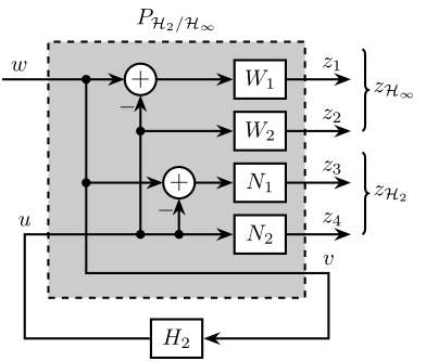
7. Mixed H2/H-Infinity Synthesis

Configuration file is accessible here.

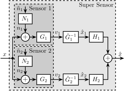
1 Sensor Fusion Architecture

\begin{tikzpicture}
  \node[branch] (x) at (0, 0);
  \node[block, above right=1.0 and 0.5 of x](G1){$G_1(s)$};
  \node[block, below right=1.0 and 0.5 of x](G2){$G_2(s)$};
  \node[addb, right=0.4 of G1](add1){};
  \node[addb, right=0.4 of G2](add2){};
  \node[block, right=1.1 of add1](H1){$H_1(s)$};
  \node[block, right=1.1 of add2](H2){$H_2(s)$};
  \node[block, above=0.5 of add1](N1){$N_1(s)$};
  \node[block, above=0.5 of add2](N2){$N_2(s)$};
  \node[addb, right=4.8 of x](add){};

  \draw[] ($(x)+(-0.7, 0)$) node[above right]{$x$} -- (x.center);
  \draw[->] (x.center) |- (G1.west);
  \draw[->] (x.center) |- (G2.west);
  \draw[->] (G1.east) -- (add1.west);
  \draw[->] (G2.east) -- (add2.west);
  \draw[->] (N1.south) -- (add1.north)node[above right]{$n_1$};
  \draw[->] (N2.south) -- (add2.north)node[above right]{$n_2$};
  \draw[<-] (N1.north) -- ++(0, 0.6)node[below right](n1){$\tilde{n}_1$};
  \draw[<-] (N2.north) -- ++(0, 0.6)node[below right](n2){$\tilde{n}_2$};
  \draw[->] (add1.east) -- (H1.west)node[above left]{$\hat{x}_1$};
  \draw[->] (add2.east) -- (H2.west)node[above left]{$\hat{x}_2$};
  \draw[->] (H1) -| (add.north);
  \draw[->] (H2) -| (add.south);
  \draw[->] (add.east) -- ++(0.7, 0) node[above left]{$\hat{x}$};

  \begin{scope}[on background layer]
    \node[fit={($(G2.south-|x)+(-0.2, -0.3)$) ($(n1.north east-|add.east)+(0.2, 0.3)$)}, fill=black!10!white, draw, dashed, inner sep=0pt] (supersensor) {};
    \node[below left] at (supersensor.north east) {Super Sensor};

    \node[fit={($(G1.south west)+(-0.3, -0.1)$) ($(n1.north east)+(0.1, 0.1)$)}, fill=black!20!white, draw, dashed, inner sep=0pt] (sensor1) {};
    \node[below right] at (sensor1.north west) {Sensor 1};
    \node[fit={($(G2.south west)+(-0.3, -0.1)$) ($(n2.north east)+(0.1, 0.1)$)}, fill=black!20!white, draw, dashed, inner sep=0pt] (sensor2) {};
    \node[below right] at (sensor2.north west) {Sensor 2};
  \end{scope}
\end{tikzpicture}

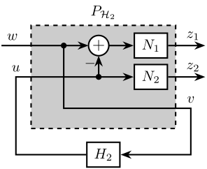
Figure 1: Sensor Fusion Architecture (png, pdf).

2 Architecture used for \(\mathcal{H}_2\) synthesis of complementary filters

\begin{tikzpicture}
   \node[block={4.0cm}{2.5cm}, fill=black!20!white, dashed] (P) {};
   \node[above] at (P.north) {$P(s)$};

   \coordinate[] (inputw)  at ($(P.south west)!0.75!(P.north west) + (-0.7, 0)$);
   \coordinate[] (inputu)  at ($(P.south west)!0.35!(P.north west) + (-0.7, 0)$);

   \coordinate[] (output1) at ($(P.south east)!0.75!(P.north east) + ( 0.7, 0)$);
   \coordinate[] (output2) at ($(P.south east)!0.35!(P.north east) + ( 0.7, 0)$);
   \coordinate[] (outputv) at ($(P.south east)!0.1!(P.north east) + ( 0.7, 0)$);

   \node[block, left=1.4 of output1] (N1){$N_1(s)$};
   \node[block, left=1.4 of output2] (N2){$N_2(s)$};
   \node[addb={+}{}{}{}{-}, left=of N1] (sub) {};

   \node[block, below=0.3 of P] (H2) {$H_2(s)$};

   \draw[->] (inputw) node[above right]{$w$} -- (sub.west);
   \draw[->] (H2.west) -| ($(inputu)+(0.35, 0)$) node[above]{$u$} -- (N2.west);
   \draw[->] (inputu-|sub) node[branch]{} -- (sub.south);
   \draw[->] (sub.east) -- (N1.west);
   \draw[->] ($(sub.west)+(-0.6, 0)$) node[branch]{} |- ($(outputv)+(-0.35, 0)$) node[above]{$v$} |- (H2.east);
   \draw[->] (N1.east) -- (output1)node[above left]{$z_1$};
   \draw[->] (N2.east) -- (output2)node[above left]{$z_2$};
\end{tikzpicture}

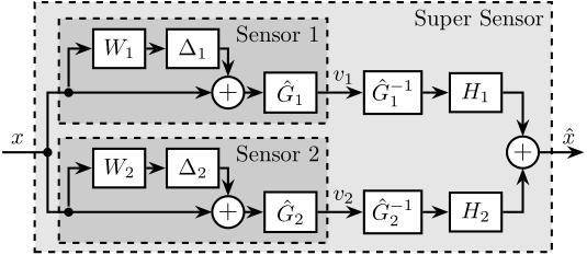
Figure 2: Architecture used for \(\mathcal{H}_\infty\) synthesis of complementary filters (png, pdf).

3 Sensor fusion architecture with sensor dynamics uncertainty

\begin{tikzpicture}
  \node[branch] (x) at (0, 0);
  \node[addb, above right=0.8 and 4 of x](add1){};
  \node[addb, below right=0.8 and 4 of x](add2){};
  \node[block, above left=0.2 and 0.1 of add1](delta1){$\Delta_1(s)$};
  \node[block, above left=0.2 and 0.1 of add2](delta2){$\Delta_2(s)$};
  \node[block, left=0.5 of delta1](W1){$w_1(s)$};
  \node[block, left=0.5 of delta2](W2){$w_2(s)$};
  \node[block, right=0.5 of add1](H1){$H_1(s)$};
  \node[block, right=0.5 of add2](H2){$H_2(s)$};
  \node[addb, right=6 of x](add){};

  \draw[] ($(x)+(-0.7, 0)$) node[above right]{$x$} -- (x.center);
  \draw[->] (x.center) |- (add1.west);
  \draw[->] (x.center) |- (add2.west);
  \draw[->] ($(add1-|W1.west)+(-0.5, 0)$)node[branch](S1){} |- (W1.west);
  \draw[->] ($(add2-|W2.west)+(-0.5, 0)$)node[branch](S1){} |- (W2.west);
  \draw[->] (W1.east) -- (delta1.west);
  \draw[->] (W2.east) -- (delta2.west);
  \draw[->] (delta1.east) -| (add1.north);
  \draw[->] (delta2.east) -| (add2.north);
  \draw[->] (add1.east) -- (H1.west);
  \draw[->] (add2.east) -- (H2.west);
  \draw[->] (H1.east) -| (add.north);
  \draw[->] (H2.east) -| (add.south);
  \draw[->] (add.east) -- ++(0.7, 0) node[above left]{$\hat{x}$};

  \begin{scope}[on background layer]
    \node[fit={($(H2.south-|x)+(-0.2, -0.3)$) ($(delta1.north east-|add.east)+(0.2, 0.4)$)}, fill=black!10!white, draw, dashed, inner sep=0pt] (supersensor) {};
    \node[below left] at (supersensor.north east) {Super Sensor};

    \node[block, fit={($(W1.north-|S1)+(-0.2, 0.2)$) ($(add1.south east)+(0.2, -0.3)$)}, fill=black!20!white, dashed, inner sep=0pt] (sensor1) {};
    \node[above right] at (sensor1.south west) {Sensor 1};
    \node[block, fit={($(W2.north-|S1)+(-0.2, 0.2)$) ($(add2.south east)+(0.2, -0.3)$)}, fill=black!20!white, dashed, inner sep=0pt] (sensor2) {};
    \node[above right] at (sensor2.south west) {Sensor 2};
  \end{scope}
\end{tikzpicture}

Figure 3: Sensor fusion architecture with sensor dynamics uncertainty (png, pdf).

4 Uncertainty set of the super sensor dynamics

\begin{tikzpicture}
  \begin{scope}[shift={(4, 0)}]

    % Uncertainty Circle
    \node[draw, circle, fill=black!20!white, minimum size=3.6cm] (c) at (0, 0) {};
    \path[draw, dotted] (0, 0) circle [radius=1.0];
    \path[draw, dashed] (135:1.0) circle [radius=0.8];

    % Center of Circle
    \node[below] at (0, 0){$1$};

    \draw[<->, dashed] (0, 0)   node[branch]{} -- coordinate[midway](r1) ++(45:1.0);
    \draw[<->, dashed] (135:1.0)node[branch]{} -- coordinate[midway](r2) ++(90:0.8);

    \node[] (l1) at (2, 1.5) {$|w_1 H_1|$};
    \draw[->, dashed, out=-90, in=0] (l1.south) to (r1);

    \node[] (l2) at (-2.5, 1.5) {$|w_2 H_2|$};
    \draw[->, dashed, out=0, in=-180] (l2.east) to (r2);

    \draw[<->, dashed] (0, 0) -- coordinate[near end](r3) ++(200:1.8);
    \node[] (l3) at (-2.5, -1.5) {$|w_1 H_1| + |w_2 H_2|$};
    \draw[->, dashed, out=90, in=-90] (l3.north) to (r3);
  \end{scope}

  % Real and Imaginary Axis
  \draw[->] (-0.5, 0) -- (7.0, 0) node[below left]{Re};
  \draw[->] (0, -1.7) -- (0, 1.7) node[below left]{Im};

  \draw[dashed] (0, 0) -- (tangent cs:node=c,point={(0, 0)},solution=2);
  \draw[dashed] (1, 0) arc (0:28:1) node[midway, right]{$\Delta \phi$};
\end{tikzpicture}

Figure 4: Uncertainty region of the super sensor dynamics in the complex plane (solid circle), of the sensor 1 (dotted circle) and of the sensor 2 (dashed circle) (png, pdf).

5 Architecture used for \(\mathcal{H}_\infty\) synthesis of complementary filters

\begin{tikzpicture}
   \node[block={4.0cm}{2.5cm}, fill=black!20!white, dashed] (P) {};
   \node[above] at (P.north) {$P(s)$};

   \coordinate[] (inputw)  at ($(P.south west)!0.75!(P.north west) + (-0.7, 0)$);
   \coordinate[] (inputu)  at ($(P.south west)!0.35!(P.north west) + (-0.7, 0)$);

   \coordinate[] (output1) at ($(P.south east)!0.75!(P.north east) + ( 0.7, 0)$);
   \coordinate[] (output2) at ($(P.south east)!0.35!(P.north east) + ( 0.7, 0)$);
   \coordinate[] (outputv) at ($(P.south east)!0.1!(P.north east) + ( 0.7, 0)$);

   \node[block, left=1.4 of output1] (W1){$W_1(s)$};
   \node[block, left=1.4 of output2] (W2){$W_2(s)$};
   \node[addb={+}{}{}{}{-}, left=of W1] (sub) {};

   \node[block, below=0.3 of P] (H2) {$H_2(s)$};

   \draw[->] (inputw) node[above right]{$w$} -- (sub.west);
   \draw[->] (H2.west) -| ($(inputu)+(0.35, 0)$) node[above]{$u$} -- (W2.west);
   \draw[->] (inputu-|sub) node[branch]{} -- (sub.south);
   \draw[->] (sub.east) -- (W1.west);
   \draw[->] ($(sub.west)+(-0.6, 0)$) node[branch]{} |- ($(outputv)+(-0.35, 0)$) node[above]{$v$} |- (H2.east);
   \draw[->] (W1.east) -- (output1)node[above left]{$z_1$};
   \draw[->] (W2.east) -- (output2)node[above left]{$z_2$};
\end{tikzpicture}

Figure 5: Architecture used for \(\mathcal{H}_\infty\) synthesis of complementary filters (png, pdf).

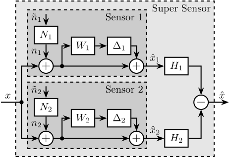
6 Sensor fusion architecture with sensor dynamics uncertainty and noise

\begin{tikzpicture}
  \node[branch] (x) at (0, 0);
  \node[addb, above right=1.2 and 3.7 of x](add1){};
  \node[addb, below right=1.2 and 3.7 of x](add2){};
  \node[block, above left=0.2 and 0.1 of add1](delta1){$\Delta_1(s)$};
  \node[block, above left=0.2 and 0.1 of add2](delta2){$\Delta_2(s)$};
  \node[block, left=0.5 of delta1](W1){$w_1(s)$};
  \node[block, left=0.5 of delta2](W2){$w_2(s)$};
  \node[addb, right=0.5 of add1](addn1){};
  \node[addb, right=0.5 of add2](addn2){};
  \node[block, above=0.5 of addn1](N1) {$N_1(s)$};
  \node[block, above=0.5 of addn2](N2) {$N_2(s)$};
  \node[block, right=1.2 of addn1](H1){$H_1(s)$};
  \node[block, right=1.2 of addn2](H2){$H_2(s)$};
  \node[addb, right=7.5 of x](add){};

  \draw[] ($(x)+(-0.7, 0)$) node[above right]{$x$} -- (x.center);
  \draw[->] (x.center) |- (add1.west);
  \draw[->] (x.center) |- (add2.west);
  \draw[->] ($(add1-|W1.west)+(-0.5, 0)$)node[branch](S1){} |- (W1.west);
  \draw[->] ($(add2-|W2.west)+(-0.5, 0)$)node[branch](S2){} |- (W2.west);
  \draw[->] (W1.east) -- (delta1.west);
  \draw[->] (W2.east) -- (delta2.west);
  \draw[->] (delta1.east) -| (add1.north);
  \draw[->] (delta2.east) -| (add2.north);
  \draw[->] (add1.east) -- (addn1.west);
  \draw[->] (add2.east) -- (addn2.west);
  \draw[->] (addn1.east) -- (H1.west)node[above left]{$\hat{x}_1$};
  \draw[->] (addn2.east) -- (H2.west)node[above left]{$\hat{x}_2$};
  \draw[->] ($(N1.north)+(0,0.7)$) node[below right](n1){$\tilde{n}_1$} -- (N1.north);
  \draw[->] ($(N2.north)+(0,0.7)$) node[below right](n2){$\tilde{n}_2$} -- (N2.north);
  \draw[->] (N1.south) -- (addn1.north)node[above right]{$n_1$};
  \draw[->] (N2.south) -- (addn2.north)node[above right]{$n_2$};
  \draw[->] (H1.east) -| (add.north);
  \draw[->] (H2.east) -| (add.south);
  \draw[->] (add.east) -- ++(0.7, 0) node[above left]{$\hat{x}$};

  \begin{scope}[on background layer]
    \node[fit={($(add2.south-|x)+(-0.2, -0.4)$) ($(n1.north-|add.east)+(0.2, 0.3)$)}, fill=black!10!white, draw, dashed, inner sep=0pt] (supersensor) {};
    \node[below left] at (supersensor.north east) {Super Sensor};
    \node[block, fit={($(S1|-add1.south)+(-0.2, -0.2)$) ($(n1.north-|N1.east)+(0.2, 0.1)$)}, fill=black!20!white, dashed, inner sep=0pt] (sensor1) {};
    \node[below right] at (sensor1.north west) {Sensor 1};
    \node[block, fit={($(S2|-add2.south)+(-0.2, -0.2)$) ($(n2.north-|N2.east)+(0.2, 0.1)$)}, fill=black!20!white, dashed, inner sep=0pt] (sensor2) {};
    \node[below right] at (sensor2.north west) {Sensor 2};
  \end{scope}
\end{tikzpicture}

Figure 6: Sensor fusion architecture with sensor dynamics uncertainty (png, pdf).

7 Mixed H2/H-Infinity Synthesis

\begin{tikzpicture}
   \node[block={5.0cm}{5.0cm}, fill=black!20!white, dashed] (P) {};
   \node[above] at (P.north) {$P(s)$};

   \coordinate[] (inputw)  at ($(P.south west)!0.85!(P.north west) + (-0.7, 0)$);
   \coordinate[] (inputu)  at ($(P.south west)!0.35!(P.north west) + (-0.7, 0)$);

   \coordinate[] (output1) at ($(P.south east)!0.85!(P.north east) + ( 0.7, 0)$);
   \coordinate[] (output2) at ($(P.south east)!0.7!(P.north east)  + ( 0.7, 0)$);
   \coordinate[] (output3) at ($(P.south east)!0.5!(P.north east)   + ( 0.7, 0)$);
   \coordinate[] (output4) at ($(P.south east)!0.35!(P.north east) + ( 0.7, 0)$);
   \coordinate[] (outputv) at ($(P.south east)!0.15!(P.north east) + ( 0.7, 0)$);

   \node[block, left=1.4 of output1] (W1){$W_1(s)$};
   \node[block, left=1.4 of output2] (W2){$W_2(s)$};
   \node[addb={+}{}{}{}{-}, left=1.6 of W1] (sub1) {};

   \node[block, left=1.4 of output3] (N1){$N_1(s)$};
   \node[block, left=1.4 of output4] (N2){$N_2(s)$};
   \node[addb={+}{}{}{}{-}, left=1 of N1] (sub2) {};

   \node[block, below=0.3 of P] (H2) {$H_2(s)$};

   \draw[->] (inputw) node[above right]{$w$} -- (sub1.west);
   \draw[->] (H2.west) -| ($(inputu)+(0.35, 0)$) node[above]{$u$} -- (N2.west);
   \draw[->] (inputu-|sub1) node[branch]{} -- (sub1.south);
   \draw[->] (inputu-|sub2) node[branch]{} -- (sub2.south);
   \draw[->] (sub1|-W2) node[branch]{} -- (W2.west);
   \draw[->] (sub1.east) -- (W1.west);
   \draw[->] (sub2.east) -- (N1.west);
   \draw[->] ($(sub1.west)+(-0.6, 0)$) node[branch](w_branch){} |- ($(outputv)+(-0.35, 0)$) node[above]{$v$} |- (H2.east);
   \draw[->] (w_branch|-sub2) node[branch]{} -- (sub2.west);
   \draw[->] (W1.east) -- (output1)node[above left]{$z_1$};
   \draw[->] (W2.east) -- (output2)node[above left]{$z_2$};
   \draw[->] (N1.east) -- (output3)node[above left]{$z_3$};
   \draw[->] (N2.east) -- (output4)node[above left]{$z_4$};
\end{tikzpicture}

Figure 7: Mixed H2/H-Infinity Synthesis (png, pdf).