Robust and Optimal Sensor Fusion - Matlab Computation
Table of Contents
- 1. Optimal Sensor Fusion for noise characteristics
- 2. Robustness to sensor dynamics uncertainty
- 3. Equivalent Super Sensor
- 4. Optimal And Robust Sensor Fusion in Practice
- 5. Methods of complementary filter synthesis
In this document, the design of complementary filters is studied.
One use of complementary filter is described below:
The basic idea of a complementary filter involves taking two or more sensors, filtering out unreliable frequencies for each sensor, and combining the filtered outputs to get a better estimate throughout the entire bandwidth of the system. To achieve this, the sensors included in the filter should complement one another by performing better over specific parts of the system bandwidth.
- in section 1, the optimal design of the complementary filters in order to obtain the lowest resulting "super sensor" noise is studied
When blending two sensors using complementary filters with unknown dynamics, phase lag may be introduced that renders the close-loop system unstable.
- in section 2, the blending robustness to sensor dynamic uncertainty is studied.
Then, three design methods for generating two complementary filters are proposed:
- in section 5.1, analytical formulas are proposed
- in section 5.2, the \(\mathcal{H}_\infty\) synthesis is used
- in section 5.3, the classical feedback architecture is used
- in section 5.4, analytical formulas found in the literature are listed
1 Optimal Sensor Fusion for noise characteristics
The idea is to combine sensors that works in different frequency range using complementary filters.
Doing so, one "super sensor" is obtained that can have better noise characteristics than the individual sensors over a large frequency range.
The complementary filters have to be designed in order to minimize the effect noise of each sensor on the super sensor noise.
All the files (data and Matlab scripts) are accessible here.
1.1 Architecture
Let's consider the sensor fusion architecture shown on figure 1 where two sensors 1 and 2 are measuring the same quantity \(x\) with different noise characteristics determined by \(W_1\) and \(W_2\).
\(n_1\) and \(n_2\) are white noise (constant power spectral density over all frequencies).

Figure 1: Fusion of two sensors
We consider that the two sensor dynamics \(G_1\) and \(G_2\) are ideal (\(G_1 = G_2 = 1\)). We obtain the architecture of figure 2.

Figure 2: Fusion of two sensors with ideal dynamics
\(H_1\) and \(H_2\) are complementary filters (\(H_1 + H_2 = 1\)). The goal is to design \(H_1\) and \(H_2\) such that the effect of the noise sources \(n_1\) and \(n_2\) has the smallest possible effect on the estimation \(\hat{x}\).
We have that the Power Spectral Density (PSD) of \(\hat{x}\) is: \[ \Gamma_{\hat{x}} = |H_1 W_1|^2 \Gamma_{n_1} + |H_2 W_2|^2 \Gamma_{n_2} \]
And the goal is the minimize the Root Mean Square (RMS) value of \(\hat{x}\): \[ \sigma_{\hat{x}} = \sqrt{\int_0^\infty \Gamma_{\hat{x}}(\omega) d\omega} \]
As \(n_1\) and \(n_2\) are white noise: \(\Gamma_{n_1} = \Gamma_{n_2} = 1\) and we have: \[ \sigma_{\hat{x}} = \sqrt{\int_0^\infty |H_1 W_1|^2(\omega) + |H_2 W_2|^2(\omega) d\omega} = \left\| \begin{matrix} H_1 W_1 \\ H_2 W_2 \end{matrix} \right\|_2 \]
Thus, the goal is to design \(H_1\) and \(H_2\) such that \(H_1 + H_2 = 1\) and such that \(\left\| \begin{matrix} H_1 W_1 \\ H_2 W_2 \end{matrix} \right\|_2\) is minimized.
For that, we will use the \(\mathcal{H}_2\) Synthesis.
1.2 Noise of the sensors
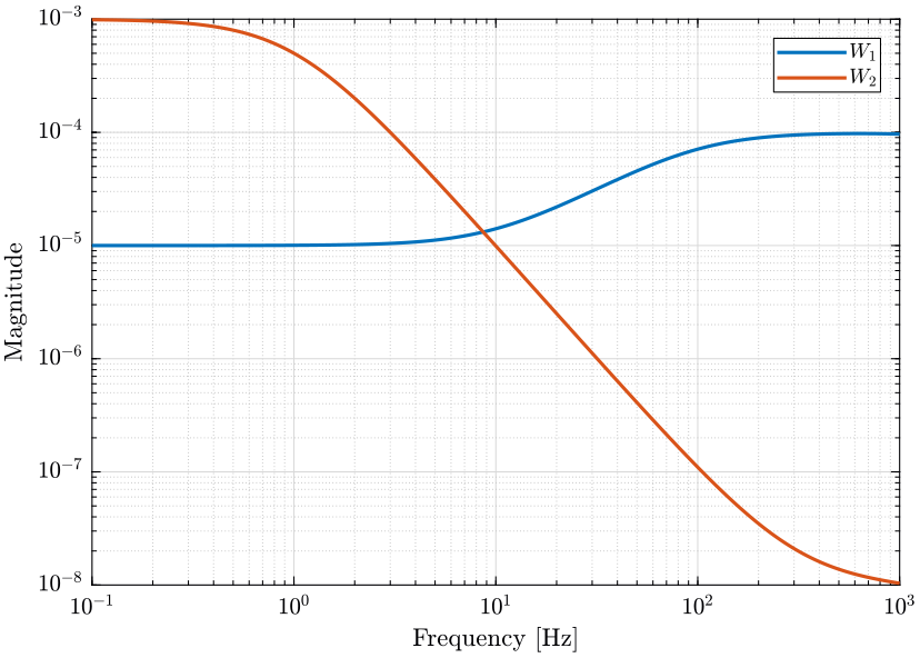
Let's define the noise characteristics of the two sensors by choosing \(W_1\) and \(W_2\):
- Sensor 1 characterized by \(W_1\) has low noise at low frequency (for instance a geophone)
- Sensor 2 characterized by \(W_2\) has low noise at high frequency (for instance an accelerometer)
omegac = 100*2*pi; G0 = 1e-5; Ginf = 1e-4;
W1 = (Ginf*s/omegac + G0)/(s/omegac + 1)/(1 + s/2/pi/4000);

omegac = 1*2*pi; G0 = 1e-3; Ginf = 1e-8;
W2 = ((sqrt(Ginf)*s/omegac + sqrt(G0))/(s/omegac + 1))^2/(1 + s/2/pi/4000)^2;
1.3 H-Two Synthesis
We use the generalized plant architecture shown on figure 4.

Figure 4: \(\mathcal{H}_2\) Synthesis - Generalized plant used for the optimal generation of complementary filters
The transfer function from \([n_1, n_2]\) to \(\hat{x}\) is: \[ \begin{bmatrix} W_1 H_1 \\ W_2 (1 - H_1) \end{bmatrix} \] If we define \(H_2 = 1 - H_1\), we obtain: \[ \begin{bmatrix} W_1 H_1 \\ W_2 H_2 \end{bmatrix} \]
Thus, if we minimize the \(\mathcal{H}_2\) norm of this transfer function, we minimize the RMS value of \(\hat{x}\).
We define the generalized plant \(P\) on matlab as shown on figure 4.
P = [0   W2  1;
     W1 -W2  0];
And we do the \(\mathcal{H}_2\) synthesis using the h2syn command.
[H1, ~, gamma] = h2syn(P, 1, 1);
What is minimized is norm([W1*H1,W2*H2], 2).
Finally, we define \(H_2 = 1 - H_1\).
H2 = 1 - H1;
1.4 Analysis
The complementary filters obtained are shown on figure 5. The PSD of the 6. Finally, the RMS value of \(\hat{x}\) is shown on table 1. The optimal sensor fusion has permitted to reduced the RMS value of the estimation error by a factor 8 compare to when using only one sensor.
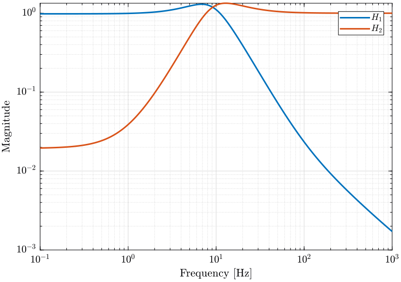
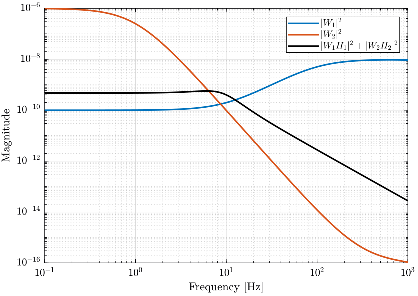
Figure 6: Power Spectral Density of the estimated \(\hat{x}\) using the two sensors alone and using the optimally fused signal (png, pdf)
| rms value | |
|---|---|
| Sensor 1 | 1.1e-02 |
| Sensor 2 | 1.3e-03 |
| Optimal Sensor Fusion | 1.5e-04 |
1.5 H-Infinity Synthesis
1.5.1 First idea
Another objective that we may have is that the noise of the super sensor \(n_{SS}\) is following the minimum of the noise of the two sensors \(n_1\) and \(n_2\): \[ \Gamma_{n_{ss}}(\omega) = \min(\Gamma_{n_1}(\omega),\ \Gamma_{n_2}(\omega)) \]
In order to obtain that ideal case, we need that the complementary filters be designed such that:
\begin{align*} & H_1(j\omega) = 1 \text{ and } H_2(j\omega) = 0 \text{ at frequencies where } \Gamma_{n_1}(\omega) < \Gamma_{n_2}(\omega) \\ & H_1(j\omega) = 0 \text{ and } H_2(j\omega) = 1 \text{ at frequencies where } \Gamma_{n_1}(\omega) > \Gamma_{n_2}(\omega) \end{align*}Which is indeed impossible in practice.
We could try to use filters with the highest possible order to approximate that. However, we may have robustness and implementation problems.
omegac = 100*2*pi; G0 = 1e-5; Ginf = 1e-4;
N1 = (Ginf*s/omegac + G0)/(s/omegac + 1)/(1 + s/2/pi/4000);

omegac = 1*2*pi; G0 = 1e-3; Ginf = 1e-8;
N2 = ((sqrt(Ginf)*s/omegac + sqrt(G0))/(s/omegac + 1))^2/(1 + s/2/pi/4000)^2;
n = 5; w0 = 2*pi*10; G0 = 1/10; G1 = 10000; Gc = 1/2;
W1 = (((1/w0)*sqrt((1-(G0/Gc)^(2/n))/(1-(Gc/G1)^(2/n)))*s + (G0/Gc)^(1/n))/((1/G1)^(1/n)*(1/w0)*sqrt((1-(G0/Gc)^(2/n))/(1-(Gc/G1)^(2/n)))*s + (1/Gc)^(1/n)))^n;

n = 5; w0 = 2*pi*8; G0 = 1000; G1 = 0.1; Gc = 1/2;
W2 = (((1/w0)*sqrt((1-(G0/Gc)^(2/n))/(1-(Gc/G1)^(2/n)))*s + (G0/Gc)^(1/n))/((1/G1)^(1/n)*(1/w0)*sqrt((1-(G0/Gc)^(2/n))/(1-(Gc/G1)^(2/n)))*s + (1/Gc)^(1/n)))^n;
P = [W1 -W1;
     0   W2;
     1   0];
And we do the \(\mathcal{H}_\infty\) synthesis using the hinfsyn command.
[H2, ~, gamma, ~] = hinfsyn(P, 1, 1,'TOLGAM', 0.001, 'METHOD', 'ric', 'DISPLAY', 'on');
[H2, ~, gamma, ~] = hinfsyn(P, 1, 1,'TOLGAM', 0.001, 'METHOD', 'ric', 'DISPLAY', 'on');
Resetting value of Gamma min based on D_11, D_12, D_21 terms

Test bounds:      0.1000 <  gamma  <=  10500.0000

  gamma    hamx_eig  xinf_eig  hamy_eig   yinf_eig   nrho_xy   p/f
1.050e+04   2.1e+01 -3.0e-07   7.8e+00   -1.3e-15    0.0000    p
5.250e+03   2.1e+01 -1.5e-08   7.8e+00   -5.8e-14    0.0000    p
2.625e+03   2.1e+01   2.5e-10   7.8e+00   -3.7e-12    0.0000    p
1.313e+03   2.1e+01 -3.2e-11   7.8e+00   -7.3e-14    0.0000    p
  656.344   2.1e+01 -2.2e-10   7.8e+00   -1.1e-15    0.0000    p
  328.222   2.1e+01 -1.1e-10   7.8e+00   -1.2e-15    0.0000    p
  164.161   2.1e+01 -2.4e-08   7.8e+00   -8.9e-16    0.0000    p
   82.130   2.1e+01   2.0e-10   7.8e+00   -9.1e-31    0.0000    p
   41.115   2.1e+01 -6.8e-09   7.8e+00   -4.1e-13    0.0000    p
   20.608   2.1e+01   3.3e-10   7.8e+00   -1.4e-12    0.0000    p
   10.354   2.1e+01 -9.8e-09   7.8e+00   -1.8e-15    0.0000    p
    5.227   2.1e+01 -4.1e-09   7.8e+00   -2.5e-12    0.0000    p
    2.663   2.1e+01   2.7e-10   7.8e+00   -4.0e-14    0.0000    p
    1.382   2.1e+01 -3.2e+05#  7.8e+00   -3.5e-14    0.0000    f
    2.023   2.1e+01 -5.0e-10   7.8e+00    0.0e+00    0.0000    p
    1.702   2.1e+01 -2.4e+07#  7.8e+00   -1.6e-13    0.0000    f
    1.862   2.1e+01 -6.0e+08#  7.8e+00   -1.0e-12    0.0000    f
    1.942   2.1e+01 -2.8e-09   7.8e+00   -8.1e-14    0.0000    p
    1.902   2.1e+01 -2.5e-09   7.8e+00   -1.1e-13    0.0000    p
    1.882   2.1e+01 -9.3e-09   7.8e+00   -2.0e-15    0.0001    p
    1.872   2.1e+01 -1.3e+09#  7.8e+00   -3.6e-22    0.0000    f
    1.877   2.1e+01 -2.6e+09#  7.8e+00   -1.2e-13    0.0000    f
    1.880   2.1e+01 -5.6e+09#  7.8e+00   -1.4e-13    0.0000    f
    1.881   2.1e+01 -1.2e+10#  7.8e+00   -3.3e-12    0.0000    f
    1.882   2.1e+01 -3.2e+10#  7.8e+00   -8.5e-14    0.0001    f

 Gamma value achieved:     1.8824
H1 = 1 - H2;
| rms value | |
|---|---|
| Sensor 1 | 1.1e-02 |
| Sensor 2 | 1.3e-03 |
| Optimal Sensor Fusion | 3.2e-04 |
1.5.2 Second idea
We have that: \[ \Phi_{n_{ss}} = \left|H_1\right|^2 \Phi_{n_1} + \left|H_2\right|^2 \Phi_{n_2} \]
We model the Power Spectral Densities of the two sensors by weighting functions \(N_1(s)\) and \(N_2(s)\). \[ \Phi_{n_{ss}} = \left|H_1 N_1\right|^2 + \left|H_2\right N_2|^2 \]
Then, at frequencies where \(|H_1| < |H_2|\) we would like that \(|N_1| = 1\) and \(|N_2| = 0\) as we discussed before. Then \(|H_1 N_1|^2 + |H_2 N_2|^2 = |H_1 N_1|^2\).
However, if we design \(H_2\) such that when \(|N_1| < |N_2|\), we have that: \[ |H_2 N_2|^2 = \epsilon |H_1 N_1|^2 \] And we have:
\begin{align*} \Phi_{n_{ss}} &= \left|H_1 N_1\right|^2 + |H_2 N_2|^2 \\ &= (1 + \epsilon)\left|H_1 N_1\right|^2 \\ &\approx \left|H_1 N_1\right|^2 \end{align*}We have then that: \[ |H_2 N_2| = \sqrt{\epsilon} |H_1 N_1| \] We suppose that \(|H_1| = 1\): \[ |H_2| = \sqrt{\epsilon} \frac{|N_1|}{|N_2|} \] We can use that for the maximum magnitude of \(|H_2|\) at frequencies where \(|N_1| < |N_2|\)
Similarly, we have that the maximum magnitude of \(|H_1|\) at frequencies where \(|N_1| > |N_2|\) is: \[ |H_1| = \sqrt{\epsilon} \frac{|N_2|}{|N_1|} \]
We could take \(\epsilon = 1\), then we increase the noise of the super sensor just by a factor \(\sqrt{2}\) over the all bandwidth from the idea case.
This could be used as weighting functions for the \(\mathcal{H}_\infty\) synthesis of the complementary filters.
omegac = 100*2*pi; G0 = 1e-5; Ginf = 1e-4;
N1 = (Ginf*s/omegac + G0)/(s/omegac + 1)/(1 + s/2/pi/4000);

omegac = 1*2*pi; G0 = 1e-3; Ginf = 1e-8;
N2 = ((sqrt(Ginf)*s/omegac + sqrt(G0))/(s/omegac + 1))^2/(1 + s/2/pi/4000)^2;
W1 = N1/N2;
W2 = N2/N1;

W1 = W1/(1 + s/2/pi/1000); % this is added so that it is proper
P = [W1 -W1;
     0   W2;
     1   0];
And we do the \(\mathcal{H}_\infty\) synthesis using the hinfsyn command.
[H2, ~, gamma, ~] = hinfsyn(P, 1, 1,'TOLGAM', 0.001, 'METHOD', 'ric', 'DISPLAY', 'on');
[H2, ~, gamma, ~] = hinfsyn(P, 1, 1,'TOLGAM', 0.001, 'METHOD', 'ric', 'DISPLAY', 'on');
Test bounds:      0.0000 <  gamma  <=   2625.0000

  gamma    hamx_eig  xinf_eig  hamy_eig   yinf_eig   nrho_xy   p/f
2.625e+03   1.8e+01 -2.3e-12   6.3e+00   -1.7e-14    0.0000    p
1.313e+03   1.8e+01 -3.3e-12   6.3e+00   -5.9e-13    0.0000    p
  656.250   1.8e+01 -1.8e-12   6.3e+00   -1.2e-13    0.0000    p
  328.125   1.8e+01 -8.3e-13   6.3e+00   -7.5e-14    0.0000    p
  164.063   1.8e+01 -3.8e-13   6.3e+00   -6.1e-14    0.0000    p
   82.031   1.8e+01 -3.3e-22   6.3e+00   -5.4e-14    0.0000    p
   41.016   1.8e+01 -3.4e-12   6.3e+00   -1.4e-16    0.0000    p
   20.508   1.8e+01 -6.4e-14   6.3e+00   -4.4e-13    0.0000    p
   10.254   1.8e+01 -1.4e-13   6.3e+00   -4.9e-14    0.0000    p
    5.127   1.7e+01 -1.1e-12   6.3e+00   -1.6e-13    0.0000    p
    2.563   1.7e+01 -6.5e-13   6.3e+00   -7.3e-14    0.0000    p
    1.282   1.4e+01 -8.9e+04#  6.3e+00   -1.6e-14    0.0000    f
    1.923   1.6e+01 -4.6e+05#  6.3e+00   -2.1e-13    0.0000    f
    2.243   1.7e+01 -1.9e+06#  6.3e+00   -9.9e-14    0.0000    f
    2.403   1.7e+01 -3.7e-11   6.3e+00   -2.1e-12    0.0000    p
    2.323   1.7e+01 -4.6e+06#  6.3e+00   -5.8e-14    0.0000    f
    2.363   1.7e+01 -1.2e+07#  6.3e+00   -3.3e-14    0.0000    f
    2.383   1.7e+01 -6.8e+07#  6.3e+00   -1.2e-13    0.0000    f
    2.393   1.7e+01 -5.5e-11   6.3e+00   -1.8e-12    0.0000    p
    2.388   1.7e+01   1.3e-22   6.3e+00   -2.5e-15    0.0000    p
    2.386   1.7e+01 -1.5e+08#  6.3e+00   -1.4e-13    0.0000    f
    2.387   1.7e+01 -4.0e+08#  6.3e+00   -1.0e-13    0.0000    f
    2.388   1.7e+01 -2.1e+09#  6.3e+00   -4.2e-13    0.0000    f

 Gamma value achieved:     2.3882
H1 = 1 - H2;
| rms value | |
|---|---|
| Sensor 1 | 1.1e-02 |
| Sensor 2 | 1.3e-03 |
| Optimal Sensor Fusion | 1.9e-04 |
1.5.3 Conclusion
From the above two experiments with \(\mathcal{H}_\infty\) it still seems that the \(\mathcal{H}_2\) synthesis gives the complementary filters that permits to obtain the minimal super sensor noise (when measuring with the \(\mathcal{H}_2\) norm)
2 Robustness to sensor dynamics uncertainty
Let's first consider ideal sensors where \(G_1 = 1\) and \(G_2 = 1\) (figure 7).

Figure 7: Fusion of two sensors
We then have:
\begin{align*} \hat{x} &= (x + n_1) H_1 + (x + n_2) H_2 \\ &= x + n_1 H_1 + n_2 H_2 \end{align*}So the estimation error is \[ \delta_x = \hat{x} - x = n_1 H_1 + n_2 H_2 \]
And we see that the complementary filters are only shaping the noise and that they do not impact the transfer function from \(x\) to \(\hat{x}\) that is in the feedback path.
All the files (data and Matlab scripts) are accessible here.
2.1 Unknown sensor dynamics dynamics
In practical systems, the sensor dynamics has always some level of uncertainty. Let's represent that with multiplicative input uncertainty as shown on figure 8.

Figure 8: Fusion of two sensors with input multiplicative uncertainty
We have:
\begin{align*} \frac{\hat{x}}{x} &= (1 + W_1 \Delta_1) H_1 + (1 + W_2 \Delta_2) H_2 \\ &= 1 + W_1 H_1 \Delta_1 + W_2 H_2 \Delta_2 \end{align*}With \(\Delta_i\) is any transfer function satisfying \(\| \Delta_i \|_\infty < 1\).
We see that as soon as we have some uncertainty in the sensor dynamics, we have that the complementary filters have some effect on the transfer function from \(x\) to \(\hat{x}\).
We want that the super sensor transfer function has a gain of 1 and no phase variation over all the frequencies: \[ \frac{\hat{x}}{x} \approx 1 \]
Thus, we want that
\begin{align*} & |W_1 H_1 \Delta_1 + W_2 H_2 \Delta_2| < \epsilon \quad \forall \omega, \forall \Delta_i, \|\Delta_i\|_\infty < 1 \\ \Longleftrightarrow & |W_1 H_1| + |W_2 H_2| < \epsilon \quad \forall \omega \end{align*}Which is approximately the same as requiring \[ \left\| \begin{matrix} W_1 H_1 \\ W_2 H_2 \end{matrix} \right\|_\infty < \epsilon \]
How small should we choose \(\epsilon\)?
The uncertainty set of the transfer function from \(\hat{x}\) to \(x\) is bounded in the complex plane by a circle centered on 1 and with a radius equal to \(\epsilon\) (figure 9).
We then have that the angle introduced by the super sensor is bounded by \(\arcsin(\epsilon)\): \[ \angle \frac{\hat{x}}{x} \le \arcsin (\epsilon) \quad \forall \omega \]

Figure 9: Maximum phase variation
Thus, we choose should choose \(\epsilon\) so that the maximum phase uncertainty introduced by the sensors is of an acceptable value.
2.2 Design the complementary filters in order to limit the phase and gain uncertainty of the super sensor
Let's say the two sensors dynamics \(H_1\) and \(H_2\) have been identified with the associated uncertainty weights \(W_1\) and \(W_2\).
If we want to have a maximum phase introduced by the sensors of 20 degrees, we have to design \(H_1\) and \(H_2\) such that:
\begin{align*} & arcsin(|H_1 W_1| + |H_2 W_2|) < 20 \text{ deg} \\ \Longleftrightarrow & |H_1 W_1| + |H_2 W_2| < 0.34 \end{align*}We can do that with the \(\mathcal{H}_\infty\) synthesis by setting upper bounds on the complementary filters using weights that corresponds to the sensor dynamics uncertainty.
For simplicity, let's suppose \(W_1(s) = W_2(s) = 0.1\) (\(10\%\) uncertainty in the sensor gain). \[ |H_1 W_1| + |H_2 W_2| < 3.4 \]
Thus, by limiting the norm of the complementary filters, we can limit the maximum unwanted phase introduced by the uncertainty on the sensors dynamics.
This is of primary importance in order to ensure the stability of the feedback loop using the super sensor signal.
2.3 First Basic Example with gain mismatch
Let's consider two ideal sensors except one sensor has not an expected gain of one but a gain of \(0.6\).
G1 = 1;
G2 = 0.6;
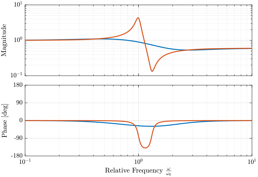
Let's design two complementary filters as shown on figure 10. The complementary filters shown in blue does not present a bump as the red ones but provides less sensor separation at high and low frequencies.
We then compute the bode plot of the super sensor transfer function \(H_1*G_1 + H_2*G_2\) for both complementary filters pair (figure 11).
We see that the blue complementary filters with a lower maximum norm permits to limit the phase lag introduced by the gain mismatch.
2.4 TODO More Complete example with model uncertainty
3 Equivalent Super Sensor
The goal here is to find the parameters of a single sensor that would best represent a super sensor.
3.1 Sensor Fusion Architecture
Let consider figure 12 where two sensors are merged. The dynamic uncertainty of each sensor is represented by a weight \(w_i(s)\), the frequency characteristics each of the sensor noise is represented by the weights \(N_i(s)\). The noise sources \(\tilde{n}_i\) are considered to be white noise: \(\Phi_{\tilde{n}_i}(\omega) = 1, \ \forall\omega\).
\begin{align*} \hat{x} &= H_1(s) N_1(s) \tilde{n}_1 + H_2(s) N_2(s) \tilde{n}_2 \\ &\quad \quad + \Big(H_1(s) \big(1 + w_1(s) \Delta_1(s)\big) + H_2(s) \big(1 + w_2(s) \Delta_2(s)\big)\Big) x \\ &= H_1(s) N_1(s) \tilde{n}_1 + H_2(s) N_2(s) \tilde{n}_2 \\ &\quad \quad + \big(1 + H_1(s) w_1(s) \Delta_1(s) + H_2(s) w_2(s) \Delta_2(s)\big) x \end{align*}To the dynamics of the super sensor is:
\begin{equation} \frac{\hat{x}}{x} = 1 + H_1(s) w_1(s) \Delta_1(s) + H_2(s) w_2(s) \Delta_2(s) \end{equation}And the noise of the super sensor is:
\begin{equation} n_{ss} = H_1(s) N_1(s) \tilde{n}_1 + H_2(s) N_2(s) \tilde{n}_2 \end{equation}3.2 Equivalent Configuration

3.3 Model the uncertainty of the super sensor
At each frequency \(\omega\), the uncertainty set of the super sensor shown on figure 12 is a circle centered on \(1\) with a radius equal to \(|H_1(j\omega) w_1(j\omega)| + |H_2(j\omega) w_2(j\omega)|\) on the complex plane. The uncertainty set of the sensor shown on figure 13 is a circle centered on \(1\) with a radius equal to \(|w_{ss}(j\omega)|\) on the complex plane.
Ideally, we want to find a weight \(w_{ss}(s)\) so that:
\[ |w_{ss}(j\omega)| = |H_1(j\omega) w_1(j\omega)| + |H_2(j\omega) w_2(j\omega)|, \quad \forall\omega \]
3.4 Model the noise of the super sensor
The PSD of the estimation \(\hat{x}\) when \(x = 0\) of the configuration shown on figure 12 is:
\begin{align*} \Phi_{\hat{x}}(\omega) &= | H_1(j\omega) N_1(j\omega) |^2 \Phi_{\tilde{n}_1} + | H_2(j\omega) N_2(j\omega) |^2 \Phi_{\tilde{n}_2} \\ &= | H_1(j\omega) N_1(j\omega) |^2 + | H_2(j\omega) N_2(j\omega) |^2 \end{align*}The PSD of the estimation \(\hat{x}\) when \(x = 0\) of the configuration shown on figure 13 is:
\begin{align*} \Phi_{\hat{x}}(\omega) &= | N_{ss}(j\omega) |^2 \Phi_{\tilde{n}} \\ &= | N_{ss}(j\omega) |^2 \end{align*}Ideally, we want to find a weight \(N_{ss}(s)\) such that:
\[ |N_{ss}(j\omega)|^2 = | H_1(j\omega) N_1(j\omega) |^2 + | H_2(j\omega) N_2(j\omega) |^2 \quad \forall\omega \]
3.5 First guess
We could choose
\begin{align*} w_{ss}(s) &= H_1(s) w_1(s) + H_2(s) w_2(s) \\ N_{ss}(s) &= H_1(s) N_1(s) + H_2(s) N_2(s) \end{align*}But we would have:
\begin{align*} |w_{ss}(j\omega)| &= |H_1(j\omega) w_1(j\omega) + H_2(j\omega) w_2(j\omega)|, \quad \forall\omega \\ &\neq |H_1(j\omega) w_1(j\omega)| + |H_2(j\omega) w_2(j\omega)|, \quad \forall\omega \end{align*}and
\begin{align*} |N_{ss}(j\omega)|^2 &= | H_1(j\omega) N_1(j\omega) + H_2(j\omega) N_2(j\omega) |^2 \quad \forall\omega \\ &\neq | H_1(j\omega) N_1(j\omega)|^2 + |H_2(j\omega) N_2(j\omega) |^2 \quad \forall\omega \\ \end{align*}4 Optimal And Robust Sensor Fusion in Practice
Here are the steps in order to apply optimal and robust sensor fusion:
- Measure the noise characteristics of the sensors to be merged (necessary for "optimal" part of the fusion)
- Measure/Estimate the dynamic uncertainty of the sensors (necessary for "robust" part of the fusion)
- Apply H2/H-infinity synthesis of the complementary filters
4.1 Measurement of the noise characteristics of the sensors
4.1.1 Huddle Test
The technique to estimate the sensor noise is taken from barzilai98_techn_measur_noise_sensor_presen.
Let's consider two sensors (sensor 1 and sensor 2) that are measuring the same quantity \(x\) as shown in figure 14.

Figure 14: Huddle test block diagram
Each sensor has uncorrelated noise \(n_1\) and \(n_2\) and internal dynamics \(G_1(s)\) and \(G_2(s)\) respectively.
We here suppose that each sensor has the same magnitude of instrumental noise: \(n_1 = n_2 = n\). We also assume that their dynamics is ideal: \(G_1(s) = G_2(s) = 1\).
We then have:
\begin{equation} \label{orgdaace50} \gamma_{\hat{x}_1\hat{x}_2}^2(\omega) = \frac{1}{1 + 2 \left( \frac{|\Phi_n(\omega)|}{|\Phi_{\hat{x}}(\omega)|} \right) + \left( \frac{|\Phi_n(\omega)|}{|\Phi_{\hat{x}}(\omega)|} \right)^2} \end{equation}Since the input signal \(x\) and the instrumental noise \(n\) are incoherent:
\begin{equation} \label{org4188c50} |\Phi_{\hat{x}}(\omega)| = |\Phi_n(\omega)| + |\Phi_x(\omega)| \end{equation}From equations \eqref{orgdaace50} and \eqref{org4188c50}, we finally obtain
4.1.2 Weights that represents the noises' PSD
For further complementary filter synthesis, it is preferred to consider a normalized noise source \(\tilde{n}\) that has a PSD equal to one (\(\Phi_{\tilde{n}}(\omega) = 1\)) and to use a weighting filter \(N(s)\) in order to represent the frequency dependence of the noise.
The weighting filter \(N(s)\) should be designed such that:
\begin{align*} & \Phi_n(\omega) \approx |N(j\omega)|^2 \Phi_{\tilde{n}}(\omega) \quad \forall \omega \\ \Longleftrightarrow & |N(j\omega)| \approx \sqrt{\Phi_n(\omega)} \quad \forall \omega \end{align*}These weighting filters can then be used to compare the noise level of sensors for the synthesis of complementary filters.
The sensor with a normalized noise input is shown in figure 15.

Figure 15: One sensor with normalized noise
4.1.3 Comparison of the noises' PSD
Once the noise of the sensors to be merged have been characterized, the power spectral density of both sensors have to be compared.
Ideally, the PSD of the noise are such that:
\begin{align*} \Phi_{n_1}(\omega) &< \Phi_{n_2}(\omega) \text{ for } \omega < \omega_m \\ \Phi_{n_1}(\omega) &> \Phi_{n_2}(\omega) \text{ for } \omega > \omega_m \end{align*}4.1.4 Computation of the coherence, power spectral density and cross spectral density of signals
The coherence between signals \(x\) and \(y\) is defined as follow \[ \gamma^2_{xy}(\omega) = \frac{|\Phi_{xy}(\omega)|^2}{|\Phi_{x}(\omega)| |\Phi_{y}(\omega)|} \] where \(|\Phi_x(\omega)|\) is the output Power Spectral Density (PSD) of signal \(x\) and \(|\Phi_{xy}(\omega)|\) is the Cross Spectral Density (CSD) of signal \(x\) and \(y\).
The PSD and CSD are defined as follow:
\begin{align} |\Phi_x(\omega)| &= \frac{2}{n_d T} \sum^{n_d}_{n=1} \left| X_k(\omega, T) \right|^2 \\ |\Phi_{xy}(\omega)| &= \frac{2}{n_d T} \sum^{n_d}_{n=1} [ X_k^*(\omega, T) ] [ Y_k(\omega, T) ] \end{align}where:
- \(n_d\) is the number for records averaged
- \(T\) is the length of each record
- \(X_k(\omega, T)\) is the finite Fourier transform of the \(k^{\text{th}}\) record
- \(X_k^*(\omega, T)\) is its complex conjugate
4.2 Estimate the dynamic uncertainty of the sensors
Let's consider one sensor represented on figure 16.
The dynamic uncertainty is represented by an input multiplicative uncertainty where \(w(s)\) is a weight that represents the level of the uncertainty.
The goal is to accurately determine \(w(s)\) for the sensors that have to be merged.

Figure 16: Sensor with dynamic uncertainty
4.3 Optimal and Robust synthesis of the complementary filters
Once the noise characteristics and dynamic uncertainty of both sensors have been determined and we have determined the following weighting functions:
- \(w_1(s)\) and \(w_2(s)\) representing the dynamic uncertainty of both sensors
- \(N_1(s)\) and \(N_2(s)\) representing the noise characteristics of both sensors
The goal is to design complementary filters \(H_1(s)\) and \(H_2(s)\) shown in figure 12 such that:
- the uncertainty on the super sensor dynamics is minimized
- the noise sources \(\tilde{n}_1\) and \(\tilde{n}_2\) has the lowest possible effect on the estimation \(\hat{x}\)

Figure 17: Sensor fusion architecture with sensor dynamics uncertainty
5 Methods of complementary filter synthesis
5.1 Complementary filters using analytical formula
All the files (data and Matlab scripts) are accessible here.
5.1.1 Analytical 1st order complementary filters
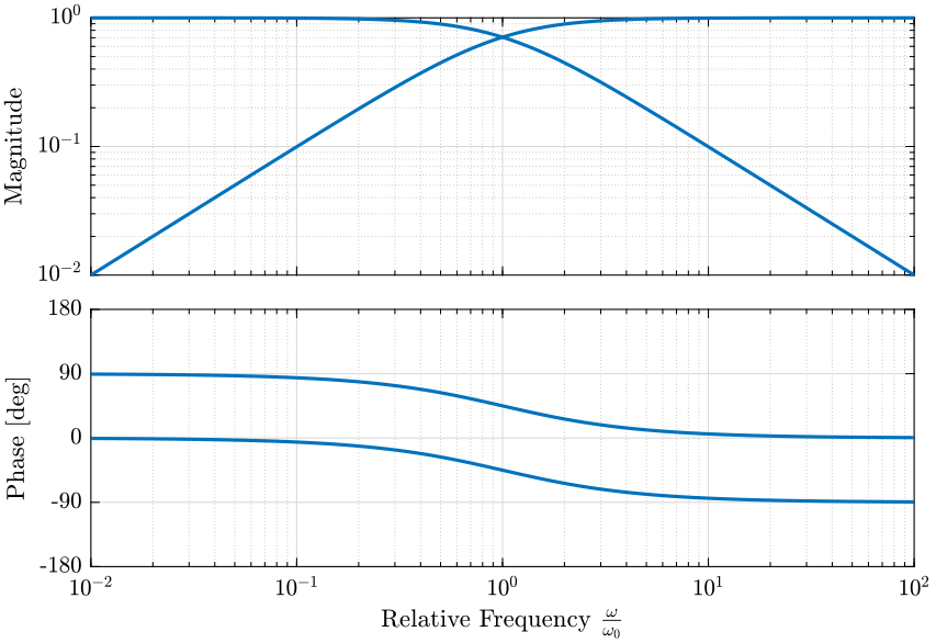
First order complementary filters are defined with following equations:
\begin{align} H_L(s) = \frac{1}{1 + \frac{s}{\omega_0}}\\ H_H(s) = \frac{\frac{s}{\omega_0}}{1 + \frac{s}{\omega_0}} \end{align}Their bode plot is shown figure 18.
w0 = 2*pi; % [rad/s]

Hh1 = (s/w0)/((s/w0)+1);
Hl1 = 1/((s/w0)+1);
5.1.2 Second Order Complementary Filters
We here use analytical formula for the complementary filters \(H_L\) and \(H_H\).
The first two formulas that are used to generate complementary filters are:
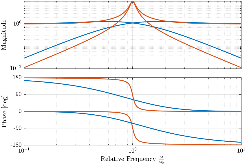
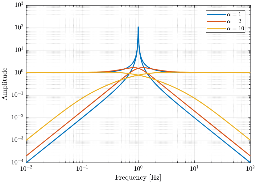
\begin{align*} H_L(s) &= \frac{(1+\alpha) (\frac{s}{\omega_0})+1}{\left((\frac{s}{\omega_0})+1\right) \left((\frac{s}{\omega_0})^2 + \alpha (\frac{s}{\omega_0}) + 1\right)}\\ H_H(s) &= \frac{(\frac{s}{\omega_0})^2 \left((\frac{s}{\omega_0})+1+\alpha\right)}{\left((\frac{s}{\omega_0})+1\right) \left((\frac{s}{\omega_0})^2 + \alpha (\frac{s}{\omega_0}) + 1\right)} \end{align*}where:
- \(\omega_0\) is the blending frequency in rad/s.
- \(\alpha\) is used to change the shape of the filters:
- Small values for \(\alpha\) will produce high magnitude of the filters \(|H_L(j\omega)|\) and \(|H_H(j\omega)|\) near \(\omega_0\) but smaller value for \(|H_L(j\omega)|\) above \(\approx 1.5 \omega_0\) and for \(|H_H(j\omega)|\) below \(\approx 0.7 \omega_0\)
- A large \(\alpha\) will do the opposite
This is illustrated on figure 19. The slope of those filters at high and low frequencies is \(-2\) and \(2\) respectively for \(H_L\) and \(H_H\).
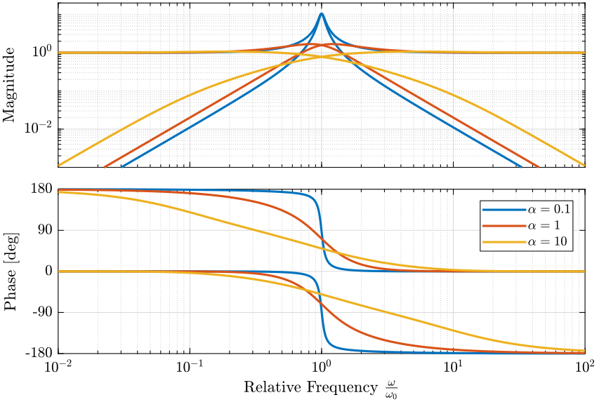
Figure 19: Effect of the parameter \(\alpha\) on the shape of the generated second order complementary filters (png, pdf)
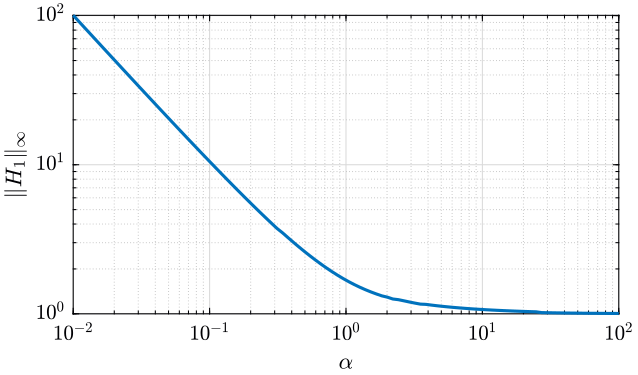
We now study the maximum norm of the filters function of the parameter \(\alpha\). As we saw that the maximum norm of the filters is important for the robust merging of filters.
figure;
plot(alphas, infnorms)
set(gca, 'xscale', 'log'); set(gca, 'yscale', 'log');
xlabel('$\alpha$'); ylabel('$\|H_1\|_\infty$');
5.1.3 Third Order Complementary Filters
The following formula gives complementary filters with slopes of \(-3\) and \(3\):
\begin{align*} H_L(s) &= \frac{\left(1+(\alpha+1)(\beta+1)\right) (\frac{s}{\omega_0})^2 + (1+\alpha+\beta)(\frac{s}{\omega_0}) + 1}{\left(\frac{s}{\omega_0} + 1\right) \left( (\frac{s}{\omega_0})^2 + \alpha (\frac{s}{\omega_0}) + 1 \right) \left( (\frac{s}{\omega_0})^2 + \beta (\frac{s}{\omega_0}) + 1 \right)}\\ H_H(s) &= \frac{(\frac{s}{\omega_0})^3 \left( (\frac{s}{\omega_0})^2 + (1+\alpha+\beta) (\frac{s}{\omega_0}) + (1+(\alpha+1)(\beta+1)) \right)}{\left(\frac{s}{\omega_0} + 1\right) \left( (\frac{s}{\omega_0})^2 + \alpha (\frac{s}{\omega_0}) + 1 \right) \left( (\frac{s}{\omega_0})^2 + \beta (\frac{s}{\omega_0}) + 1 \right)} \end{align*}The parameters are:
- \(\omega_0\) is the blending frequency in rad/s
- \(\alpha\) and \(\beta\) that are used to change the shape of the filters similarly to the parameter \(\alpha\) for the second order complementary filters
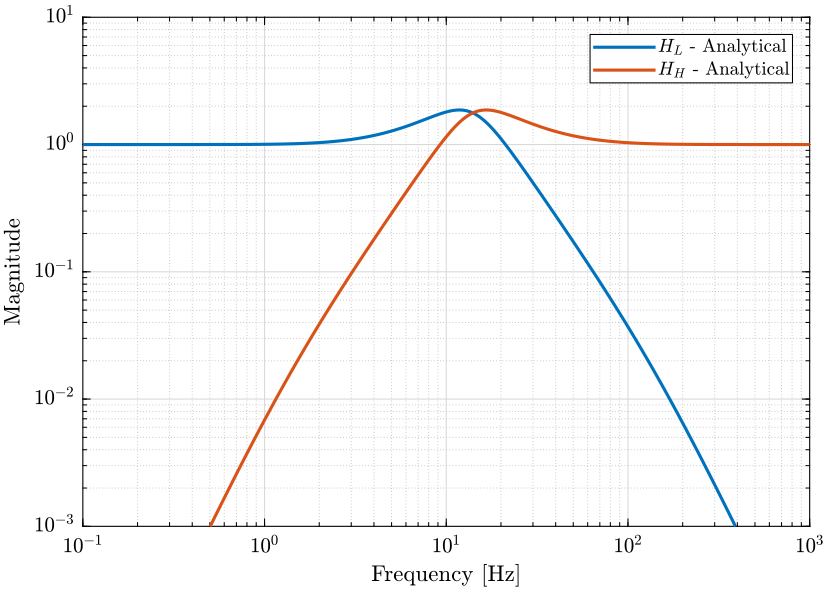
The filters are defined below and the result is shown on figure 21.
alpha = 1;
beta = 10;
w0 = 2*pi*14;

Hh3_ana = (s/w0)^3 * ((s/w0)^2 + (1+alpha+beta)*(s/w0) + (1+(alpha+1)*(beta+1)))/((s/w0 + 1)*((s/w0)^2+alpha*(s/w0)+1)*((s/w0)^2+beta*(s/w0)+1));
Hl3_ana = ((1+(alpha+1)*(beta+1))*(s/w0)^2 + (1+alpha+beta)*(s/w0) + 1)/((s/w0 + 1)*((s/w0)^2+alpha*(s/w0)+1)*((s/w0)^2+beta*(s/w0)+1));
5.2 H-Infinity synthesis of complementary filters
All the files (data and Matlab scripts) are accessible here.
5.2.1 Synthesis Architecture
We here synthesize the complementary filters using the \(\mathcal{H}_\infty\) synthesis. The goal is to specify upper bounds on the norms of \(H_L\) and \(H_H\) while ensuring their complementary property (\(H_L + H_H = 1\)).
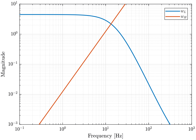
In order to do so, we use the generalized plant shown on figure 22 where \(w_L\) and \(w_H\) weighting transfer functions that will be used to shape \(H_L\) and \(H_H\) respectively.

Figure 22: Generalized plant used for the \(\mathcal{H}_\infty\) synthesis of the complementary filters
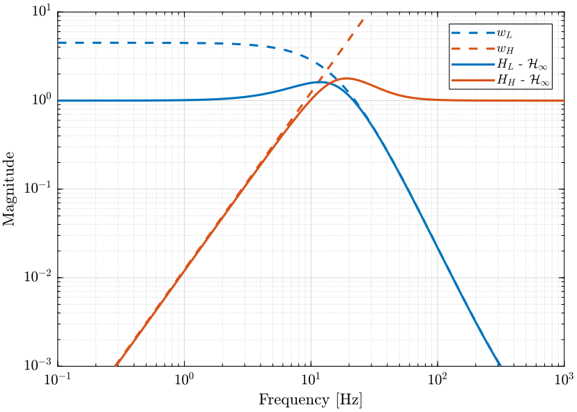
The \(\mathcal{H}_\infty\) synthesis applied on this generalized plant will give a transfer function \(H_L\) (figure 23) such that the \(\mathcal{H}_\infty\) norm of the transfer function from \(w\) to \([z_H,\ z_L]\) is less than one: \[ \left\| \begin{array}{c} H_L w_L \\ (1 - H_L) w_H \end{array} \right\|_\infty < 1 \]
Thus, if the above condition is verified, we can define \(H_H = 1 - H_L\) and we have that: \[ \left\| \begin{array}{c} H_L w_L \\ H_H w_H \end{array} \right\|_\infty < 1 \] Which is almost (with an maximum error of \(\sqrt{2}\)) equivalent to:
\begin{align*} |H_L| &< \frac{1}{|w_L|}, \quad \forall \omega \\ |H_H| &< \frac{1}{|w_H|}, \quad \forall \omega \end{align*}We then see that \(w_L\) and \(w_H\) can be used to shape both \(H_L\) and \(H_H\) while ensuring (by definition of \(H_H = 1 - H_L\)) their complementary property.

Figure 23: \(\mathcal{H}_\infty\) synthesis of the complementary filters
5.2.2 Weights
5.2.3 H-Infinity Synthesis
We define the generalized plant \(P\) on matlab.
P = [0   wL;
     wH -wH;
     1   0];
And we do the \(\mathcal{H}_\infty\) synthesis using the hinfsyn command.
[Hl_hinf, ~, gamma, ~] = hinfsyn(P, 1, 1,'TOLGAM', 0.001, 'METHOD', 'ric', 'DISPLAY', 'on');
[Hl_hinf, ~, gamma, ~] = hinfsyn(P, 1, 1,'TOLGAM', 0.001, 'METHOD', 'ric', 'DISPLAY', 'on');
Test bounds:      0.0000 <  gamma  <=      1.7285

  gamma    hamx_eig  xinf_eig  hamy_eig   yinf_eig   nrho_xy   p/f
    1.729   4.1e+01   8.4e-12   1.8e-01    0.0e+00    0.0000    p
    0.864   3.9e+01 -5.8e-02#  1.8e-01    0.0e+00    0.0000    f
    1.296   4.0e+01   8.4e-12   1.8e-01    0.0e+00    0.0000    p
    1.080   4.0e+01   8.5e-12   1.8e-01    0.0e+00    0.0000    p
    0.972   3.9e+01 -4.2e-01#  1.8e-01    0.0e+00    0.0000    f
    1.026   4.0e+01   8.5e-12   1.8e-01    0.0e+00    0.0000    p
    0.999   3.9e+01   8.5e-12   1.8e-01    0.0e+00    0.0000    p
    0.986   3.9e+01 -1.2e+00#  1.8e-01    0.0e+00    0.0000    f
    0.993   3.9e+01 -8.2e+00#  1.8e-01    0.0e+00    0.0000    f
    0.996   3.9e+01   8.5e-12   1.8e-01    0.0e+00    0.0000    p
    0.994   3.9e+01   8.5e-12   1.8e-01    0.0e+00    0.0000    p
    0.993   3.9e+01 -3.2e+01#  1.8e-01    0.0e+00    0.0000    f

 Gamma value achieved:     0.9942
We then define the high pass filter \(H_H = 1 - H_L\). The bode plot of both \(H_L\) and \(H_H\) is shown on figure 25.
Hh_hinf = 1 - Hl_hinf;
5.3 Feedback Control Architecture to generate Complementary Filters
The idea is here to use the fact that in a classical feedback architecture, \(S + T = 1\), in order to design complementary filters.
Thus, all the tools that has been developed for classical feedback control can be used for complementary filter design.
All the files (data and Matlab scripts) are accessible here.
5.3.1 Architecture

Figure 26: Architecture used to generate the complementary filters
We have: \[ y = \underbrace{\frac{L}{L + 1}}_{H_L} y_1 + \underbrace{\frac{1}{L + 1}}_{H_H} y_2 \] with \(H_L + H_H = 1\).
The only thing to design is \(L\) such that the complementary filters are stable with the wanted shape.
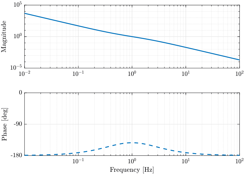
A simple choice is: \[ L = \left(\frac{\omega_c}{s}\right)^2 \frac{\frac{s}{\omega_c / \alpha} + 1}{\frac{s}{\omega_c} + \alpha} \]
Which contains two integrator and a lead. \(\omega_c\) is used to tune the crossover frequency and \(\alpha\) the trade-off "bump" around blending frequency and filtering away from blending frequency.
5.3.2 Loop Gain Design
5.4 Analytical Formula found in the literature
5.4.1 Analytical Formula
min15_compl_filter_desig_angle_estim
\begin{align*} H_L(s) = \frac{K_p s + K_i}{s^2 + K_p s + K_i} \\ H_H(s) = \frac{s^2}{s^2 + K_p s + K_i} \end{align*}corke04_inert_visual_sensin_system_small_auton_helic
\begin{align*} H_L(s) = \frac{1}{s/p + 1} \\ H_H(s) = \frac{s/p}{s/p + 1} \end{align*} \begin{align*} H_L(s) = \frac{2 \omega_0 s + \omega_0^2}{(s + \omega_0)^2} \\ H_H(s) = \frac{s^2}{(s + \omega_0)^2} \end{align*} \begin{align*} H_L(s) = \frac{C(s)}{C(s) + s} \\ H_H(s) = \frac{s}{C(s) + s} \end{align*} \begin{align*} H_L(s) = \frac{3 \tau s + 1}{(\tau s + 1)^3} \\ H_H(s) = \frac{\tau^3 s^3 + 3 \tau^2 s^2}{(\tau s + 1)^3} \end{align*} \begin{align*} H_L(s) = \frac{2 \tau s + 1}{(\tau s + 1)^2} \\ H_H(s) = \frac{\tau^2 s^2}{(\tau s + 1)^2} \end{align*}5.4.2 Matlab
omega0 = 1*2*pi; % [rad/s]
tau = 1/omega0; % [s]

% From cite:corke04_inert_visual_sensin_system_small_auton_helic
HL1 = 1/(s/omega0 + 1); HH1 = s/omega0/(s/omega0 + 1);

% From cite:jensen13_basic_uas
HL2 = (2*omega0*s + omega0^2)/(s+omega0)^2; HH2 = s^2/(s+omega0)^2;

% From cite:shaw90_bandw_enhan_posit_measur_using_measur_accel
HL3 = (3*tau*s + 1)/(tau*s + 1)^3; HH3 = (tau^3*s^3 + 3*tau^2*s^2)/(tau*s + 1)^3;

5.4.3 Discussion
Analytical Formula found in the literature provides either no parameter for tuning the robustness / performance trade-off.
5.5 Comparison of the different methods of synthesis
The generated complementary filters using \(\mathcal{H}_\infty\) and the analytical formulas are very close to each other. However there is some difference to note here:
- the analytical formula provides a very simple way to generate the complementary filters (and thus the controller), they could even be used to tune the controller online using the parameters \(\alpha\) and \(\omega_0\). However, these formula have the property that \(|H_H|\) and \(|H_L|\) are symmetrical with the frequency \(\omega_0\) which may not be desirable.
- while the \(\mathcal{H}_\infty\) synthesis of the complementary filters is not as straightforward as using the analytical formula, it provides a more optimized procedure to obtain the complementary filters
Bibliography
- [barzilai98_techn_measur_noise_sensor_presen] Aaron Barzilai, Tom VanZandt & Tom Kenny, Technique for Measurement of the Noise of a Sensor in the Presence of Large Background Signals, Review of Scientific Instruments, 69(7), 2767-2772 (1998). link. doi.
- [min15_compl_filter_desig_angle_estim] Min & Jeung, Complementary Filter Design for Angle Estimation Using Mems Accelerometer and Gyroscope, Department of Control and Instrumentation, Changwon National University, Changwon, Korea, 641-773 (2015).
- [corke04_inert_visual_sensin_system_small_auton_helic] Peter Corke, An Inertial and Visual Sensing System for a Small Autonomous Helicopter, Journal of Robotic Systems, 21(2), 43-51 (2004). link. doi.
- [jensen13_basic_uas] Austin Jensen, Cal Coopmans & YangQuan Chen, Basics and guidelines of complementary filters for small UAS navigation, nil, in in: 2013 International Conference on Unmanned Aircraft Systems (ICUAS), edited by (2013)
- [shaw90_bandw_enhan_posit_measur_using_measur_accel] Shaw & Srinivasan, Bandwidth Enhancement of Position Measurements Using Measured Acceleration, Mechanical Systems and Signal Processing, 4(1), 23-38 (1990). link. doi.
- [baerveldt97_low_cost_low_weigh_attit] Baerveldt & Klang, A Low-Cost and Low-Weight Attitude Estimation System for an Autonomous Helicopter, nil, in in: Proceedings of IEEE International Conference on Intelligent Engineering Systems, edited by (1997)