Attocube - Test Bench

1. Estimation of the Spectral Density of the Attocube Noise
2. Effect of the “bubble sheet” and Aluminium tube

1 Estimation of the Spectral Density of the Attocube Noise

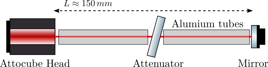
Figure 1: Test Bench Schematic

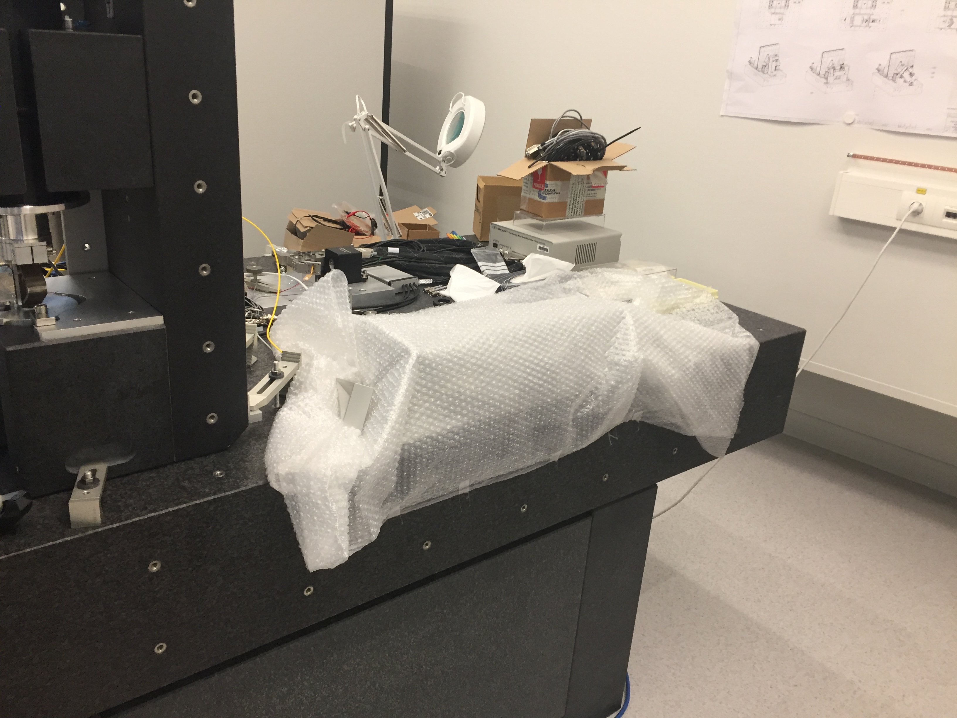
Figure 2: Picture of the test bench. The Attocube and mirror are covered by a “bubble sheet”

1.1 Long and Slow measurement

The first measurement was made during ~17 hours with a sampling time of \(T_s = 0.1\,s\).

load('./mat/long_test2.mat', 'x', 't')
Ts = 0.1; % [s]

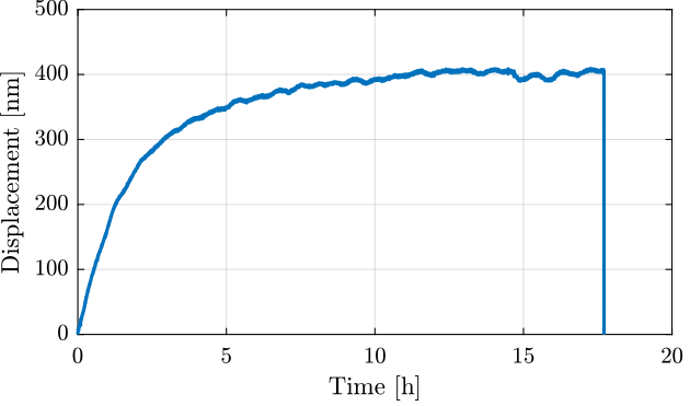
Figure 3: Long measurement time domain data

Let’s fit the data with a step response to a first order low pass filter (Figure 4).

f = @(b,x) b(1)*(1 - exp(-x/b(2)));

y_cur = x(t < 17*60*60);
t_cur = t(t < 17*60*60);

nrmrsd = @(b) norm(y_cur - f(b,t_cur)); % Residual Norm Cost Function
B0 = [400e-9, 2*60*60];                        % Choose Appropriate Initial Estimates
[B,rnrm] = fminsearch(nrmrsd, B0);     % Estimate Parameters ‘B’

The corresponding time constant is (in [h]):

2.0576

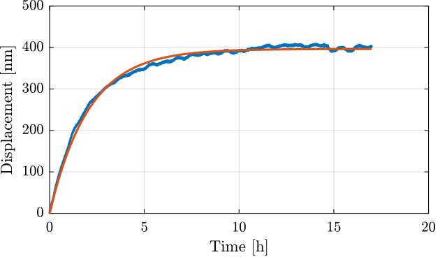
Figure 4: Fit of the measurement data with a step response of a first order low pass filter

We can see in Figure 3 that there is a transient period where the measured displacement experiences some drifts. This is probably due to thermal effects. We only select the data between t1 and t2. The obtained displacement is shown in Figure 5.

t1 = 11; t2 = 17; % [h]

x = x(t > t1*60*60 & t < t2*60*60);
x = x - mean(x);
t = t(t > t1*60*60 & t < t2*60*60);
t = t - t(1);

Figure 5: Kept data (removed slow drifts during the first hours)

The Power Spectral Density of the measured displacement is computed

win = hann(ceil(length(x)/20));
[p_1, f_1] = pwelch(x, win, [], [], 1/Ts);

As a low pass filter was used in the measurement process, we multiply the PSD by the square of the inverse of the filter’s norm.

G_lpf = 1/(1 + s/2/pi);
p_1 = p_1./abs(squeeze(freqresp(G_lpf, f_1, 'Hz'))).^2;

Only frequencies below 2Hz are taken into account (high frequency noise will be measured afterwards).

p_1 = p_1(f_1 < 2);
f_1 = f_1(f_1 < 2);

1.2 Short and Fast measurement

An second measurement is done in order to estimate the high frequency noise of the interferometer. The measurement is done with a sampling time of \(T_s = 0.1\,ms\) and a duration of ~100s.

load('./mat/short_test_plastic.mat')
Ts = 1e-4; % [s]

x = detrend(x, 0);

The time domain measurement is shown in Figure 6.

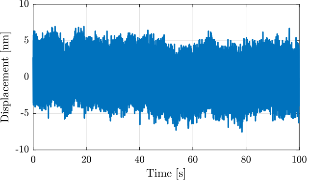
Figure 6: Time domain measurement with the high sampling rate

The Power Spectral Density of the measured displacement is computed

win = hann(ceil(length(x)/10));
[p_2, f_2] = pwelch(x, win, [], [], 1/Ts);

1.3 Obtained Amplitude Spectral Density of the measured displacement

The computed ASD of the two measurements are combined in Figure 7.

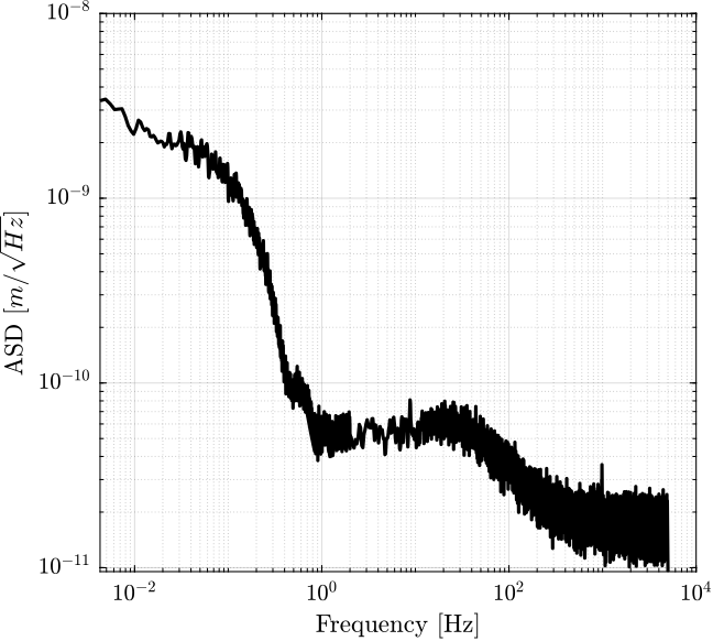
Figure 7: Obtained Amplitude Spectral Density of the measured displacement

2 Effect of the “bubble sheet” and Aluminium tube

Figure 8: Aluminium tube used to protect the beam path from disturbances

2.1 Aluminium Tube and Bubble Sheet

load('./mat/long_test_plastic.mat');
Ts = 1e-4; % [s]

x = detrend(x, 0);

win = hann(ceil(length(x)/10));
[p_1, f_1] = pwelch(x, win, [], [], 1/Ts);

2.2 Only Aluminium Tube

load('./mat/long_test_alu_tube.mat');
Ts = 1e-4; % [s]

x = detrend(x, 0);